This article explains multiple ways to lookup a value based on multiple criteria or conditions in Excel.
Suppose you have data in Excel for students' first names with their sections and final scores. You are asked to find the score of a student given its name and section.
Please click on the link below to download the Excel file used for explaining this article.
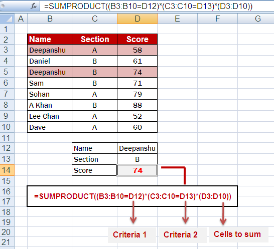
=SUMPRODUCT((B3:B10=D12)*(C3:C10=D13)*(D3:D10))
- B3:D10 : Range in which you want to apply the first criteria (i.e. Name).
- C3:D10 : Range in which you want to apply the second criteria (i.e. Section).
- D3:D10 : Range from which you want to extract the desired value (i.e. section).
- D12 : Criteria 1 (i.e. Name).
- D13 : Criteria 2 (i.e. Section).
The formula checks if cells in B3:B10 match the criteria in D12 (Name) and C3:C10 match D13 (Section). It creates TRUE/FALSE arrays. These arrays are multiplied with D3:D10, summed up and returns the matching value from D3:D10 range (i.e. student's score).
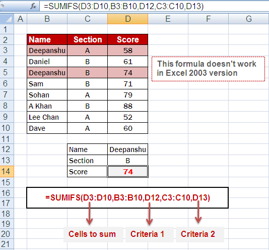
=SUMIFS(D3:D10,B3:B10,D12,C3:C10,D13)
This SUMIFS formula returns the value from the range D3:D10 that meet multiple conditions i.e. (B3:B10 = D12) and (C3:C10 = D13).
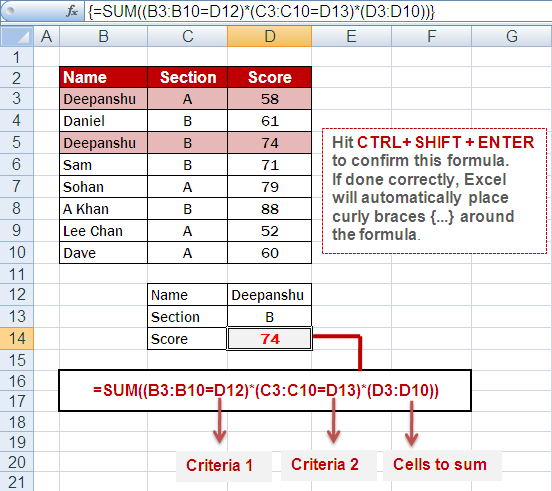
=SUM((B3:B10=D12)*(C3:C10=D13)*(D3:D10))
Hit CTRL+ SHIFT + ENTER to confirm this formula instead of the usual ENTER key as it is an array formula. If done correctly, Excel will automatically place curly braces {...} around the formula.
After placing curly braces, the formula would look like this in formula bar :
{=SUM((B3:B10=D12)*(C3:C10=D13)*(D3:D10))}
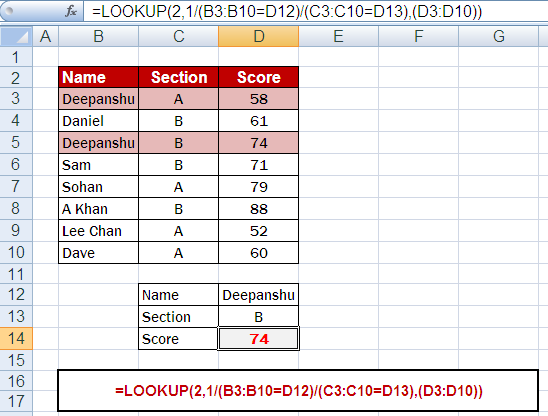
=LOOKUP(2,1/(B3:B10=D12)/(C3:C10=D13),(D3:D10))
The formula searches for the value "2" in the array created by dividing 1 by the conditions (B3:B10=D12) and (C3:C10=D13). It then returns the corresponding value from the range D3:D10. This formula performs a reverse lookup to find the last value that matches the specified criteria.
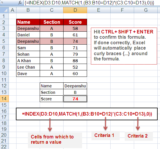
=INDEX(D3:D10,MATCH(1,(B3:B10=D12)*(C3:C10=D13),0))
Hit CTRL+ SHIFT + ENTER to confirm this formula. If done correctly, Excel will automatically place curly braces {...} around the formula.
The formula pulls the value from the range D3:D10 that meets the criteria specified. It uses the MATCH function to find the position of the first occurrence of "1" in the array created by multiplying (B3:B10=D12) and (C3:C10=D13). The INDEX function then returns the corresponding value from the range D3:D10 at that position.
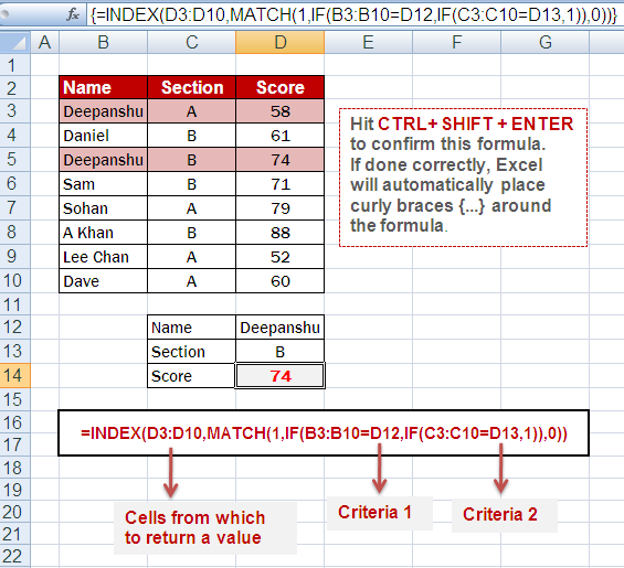
=INDEX(D3:D10,MATCH(1,IF(B3:B10=D12,IF(C3:C10=D13,1)),0))
Hit CTRL+ SHIFT + ENTER to confirm this formula as it's an array formula.
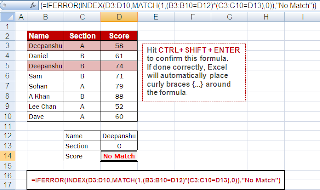
=IFERROR(INDEX(D3:D10,MATCH(1,(B3:B10=D12)*(C3:C10=D13),0)),"No Match")
This formula returns "No Match" if no value exists on the basis of conditions. Press CTRL+ SHIFT + ENTER to confirm this array formula.


WHAT IF STUDENT BELONG FROM SAME SECTION AND SAME FIRST NAME.?
ReplyDeletePREMLATA2733@GMAIL.COM
ReplyDeletePROVIDE THE EXCEL SHEET
Thank you! What a big help!
ReplyDeleteThe explanation of 4. INDEX-MATCH was exactly what I was looking for - works great when comparing 2 conditions in different worksheets and returning a third value
ReplyDelete