This tutorial explains how to find the smallest value in Excel based on a single or multiple conditions.
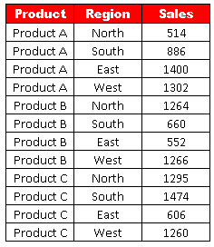
Suppose you have data for products, sales and regions. You are asked to figure out the minimum sales generated by Product B. The data is shown in the image below.

Download the workbook
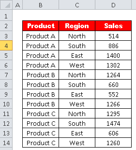
Assuming you have data in range B3:D14. (See the image below)

To calculate the minimum sales generated by Product B.
=MIN(IF(B3:B14="Product B",D3:D14))Since the above formula is an array formula, press CTRL SHIFT ENTER to confirm it instead of simply pressing the ENTER key.
After pressing CTRL SHIFT ENTER, the formula will be surrounded by curly braces. It will look like:
{=MIN(IF(B3:B14="Product B",D3:D14))}
B3:B14: It represents the cells B3 to B14, which contains product information."Product B": This is the condition being tested. It checks if the corresponding cells in the rangeB3:B14contain the text"Product B".D3:D14: It represents the cells D3 to D14, which contains sales figure related to the products mentioned in column B.IF(B3:B14="Product B",D3:D14): This part of the formula creates an array of values. It goes through each cell in the rangeB3:B14and checks if the corresponding cell contains the text"Product B". If it does, it returns the value from the corresponding cell in the rangeD3:D14. Otherwise, it returnsFALSEor an error.MIN(IF(B3:B14="Product B",D3:D14)): Finally, theMINfunction is used to find the minimum value from the array of values created by theIFfunction. It will identify the smallest value among the numbers returned by theIFfunction, which is the minimum value in column D (D3:D14) where the corresponding cell in column B (B3:B14) contains"Product B".
Find the Minimum Value in Excel with Multiple Criteria
To calculate the minimum sales generated by Product B in East region.

=MIN(IF((B3:B14="Product B")*(C3:C14="East"),D3:D14))Since the above formula is an array formula, press CTRL SHIFT ENTER to confirm it instead of simply pressing the ENTER key.
After pressing CTRL SHIFT ENTER, the formula will be surrounded by curly braces. It will look like:
{=MIN(IF((B3:B14="Product B")*(C3:C14="East"),D3:D14))}
(B3:B14="Product B")*(C3:C14="East"): This part of the formula combines the two conditions using multiplication. The * (asterisk) acts as the AND operator in array formulas. So, this expression creates an array of TRUE and FALSE values, where each element corresponds to whether the conditions are met for the corresponding row.IF((B3:B14="Product B")*(C3:C14="East"),D3:D14): This part of the formula creates another array of values. It goes through each cell in the range B3:B14 and C3:C14 and checks if both conditions are true for that row. If both conditions are true, it returns the value from the corresponding cell in the range D3:D14. Otherwise, it returns FALSE or an error.MIN(IF((B3:B14="Product B")*(C3:C14="East"),D3:D14)): Finally, theMINfunction is used to find the minimum value from the array of values created by theIFfunction. It will identify the smallest value among the numbers returned by theIFfunction, which is the minimum value in column D (D3:D14) where the corresponding cells in columns B and C (B3:B14 and C3:C14) meet the specified conditions ("Product B" in column B and "East" in column C).


Share Share Tweet