Logistic Regression
It is used to predict the result of a categorical dependent variable based on one or more continuous or categorical independent variables. In other words, it is multiple regression analysis but with a dependent variable is categorical.
Examples
1. An employee may get promoted or not based on age, years of experience, last performance rating etc. We are trying to calculate the factors that affects promotion. In this case, two possible categories in dependent variable : "Promoted" and "Not Promoted".
2. We are interested in knowing how variables, such as age, sex, body mass index, effect blood pressure (sbp). In this case, two possible categories in dependent variable : "High Blood Pressure" and "Normal Blood Pressure".
Algorithm
Logistic regression is based on Maximum Likelihood (ML) Estimation which says coefficients should be chosen in such a way that it maximizes the Probability of Y given X (likelihood). With ML, the computer uses different "iterations" in which it tries different solutions until it gets the maximum likelihood estimates. Fisher Scoring is the most popular iterative method of estimating the regression parameters.
Take exponential both the sides
Distribution
Interpretation of Logistic Regression Estimates
If X increases by one unit, the log-odds of Y increases by k unit, given the other variables in the model are held constant.
In logistic regression, the odds ratio is easier to interpret. That is also called Point estimate. It is exponential value of estimate.
For Continuous Predictor
Magnitude : If you want to compare the magnitudes of positive and negative effects, simply take the inverse of the negative effects. For example, if Exp(B) = 2 on a positive effect variable, this has the same magnitude as variable with Exp(B) = 0.5 = ½ but in the opposite direction.
It looks at maximum difference between distribution of cumulative events and cumulative non-events.
Interpret Results :
1. Odd Ratio of GPA (Exp value of GPA Estimate) = 3.196 implies for a one unit increase in GPA, the odds of being admitted to graduate school increase by a factor of 3.196.
It is used to predict the result of a categorical dependent variable based on one or more continuous or categorical independent variables. In other words, it is multiple regression analysis but with a dependent variable is categorical.
Examples
1. An employee may get promoted or not based on age, years of experience, last performance rating etc. We are trying to calculate the factors that affects promotion. In this case, two possible categories in dependent variable : "Promoted" and "Not Promoted".
2. We are interested in knowing how variables, such as age, sex, body mass index, effect blood pressure (sbp). In this case, two possible categories in dependent variable : "High Blood Pressure" and "Normal Blood Pressure".
Algorithm
Logistic regression is based on Maximum Likelihood (ML) Estimation which says coefficients should be chosen in such a way that it maximizes the Probability of Y given X (likelihood). With ML, the computer uses different "iterations" in which it tries different solutions until it gets the maximum likelihood estimates. Fisher Scoring is the most popular iterative method of estimating the regression parameters.
logit(p) = b0 + b1X1 + b2X2 + ------ + bk Xkwhere logit(p) = loge(p / (1-p))
Take exponential both the sides
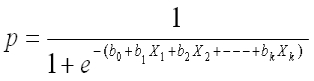 |
| Logistic Regression Equation |
p : the probability of the dependent variable equaling a "success" or "event".
 |
| Logistic Regression Curve |
Distribution
Binary logistic regression model assumes binomial distribution of the response with N(number of trials) and p(probability of success). Logistic regression is in the 'binomial family' of GLMs. The dependent variable does not need to be normally distributed.Example - If you flip a coin twice, what is the probability of getting one or more heads? It's a binomial distribution with N=2 and p=0.5. The binomial distribution consists of the probabilities of each of the possible numbers of successes on N trials for independent events that each have a probability of p.
Interpretation of Logistic Regression Estimates
If X increases by one unit, the log-odds of Y increases by k unit, given the other variables in the model are held constant.
For Continuous Predictor
An unit increase in years of experience increases the odds of getting a job by a multiplicative factor of 4.27, given the other variables in the model are held constant. In other words, the odds of getting a job are increased by 327% (4.27-1)*100 for an unit increase in years of experience.For Binary Predictor
The odds of a person having years of experience getting a job are 4.27 times greater than the odds of a person having no experience.Note : To calculate 5 unit increase, 4.27 ^ 5 (instead of multiplication).
Magnitude : If you want to compare the magnitudes of positive and negative effects, simply take the inverse of the negative effects. For example, if Exp(B) = 2 on a positive effect variable, this has the same magnitude as variable with Exp(B) = 0.5 = ½ but in the opposite direction.
Odd Ratio (exp of estimate) less than 1 ==> Negative relationship (It means negative coefficient value of estimate coefficients)
Test Overall Fit of the Model : -2 Log L , Score and Wald Chi-Square
These are Chi-Square tests. They test against the null hypothesis that at least one of the predictors' regression coefficient is not equal to zero in the model.
Assumptions of Logistic Regression
- The logit transformation of the outcome variable has a linear relationship with the predictor variables. The one way to check the assumption is to categorize the independent variables. Transform the numeric variables to 10/20 groups and then check whether they have linear or monotonic relationship.
- No multicollinearity problem. No high correlationship between predictors.
- No influential observations (Outliers).
- Large Sample Size - It requires atleast 10 events per independent variable.
Important Performance Metrics
1. Percent Concordant : Percentage of pairs where the observation with the desired outcome (event) has a higher predicted probability than the observation without the outcome (non-event).
Rule: Higher the percentage of concordant pairs the better is the fit of the model. Above 80% considered good model.
2. Percent Discordant : Percentage of pairs where the observation with the desired outcome (event) has a lower predicted probability than the observation without the outcome (non-event).
3. Percent Tied : Percentage of pairs where the observation with the desired outcome (event) has same predicted probability than the observation without the outcome (non-event).
4. Area under curve (c statistics) - It ranges from 0.5 to 1, where 0.5 corresponds to the model randomly predicting the response, and a 1 corresponds to the model perfectly discriminating the response.
C = Area under Curve = %concordant + (0.5 * %tied)
.90-1 = excellent (A)
.80-.90 = good (B)
.70-.80 = fair (C)
.60-.70 = poor (D)
.50-.60 = fail (F)
5. Classification Table (Confusion Matrix)
Sensitivity (True Positive Rate) - % of events of dependent variable successfully predicted as events.
Sensitivity = TRUE POS / (TRUE POS + FALSE NEG)
Specificity (True Negative Rate) - % of non-events of dependent variable successfully predicted as non-events.
Specificity = TRUE NEG / (TRUE NEG + FALSE POS)
Correct (Accuracy) = Number of correct prediction (TRUE POS + TRUE NEG) divided by sample size.
6. KS Statistics
Detailed Explanation - How to Check Model Performance
Problem Statement -
A researcher is interested in how variables, such as GRE (Graduate Record Exam scores), GPA (grade point average) and prestige of the undergraduate institution, affect admission into graduate school. The outcome variable, admit/don't admit, is binary.
This data set has a binary response (outcome, dependent) variable called admit, which is equal to 1 if the individual was admitted to graduate school, and 0 otherwise. There are three predictor variables: gre, gpa, and rank. We will treat the variables gre and gpa as continuous. The variable rank takes on the values 1 through 4. Institutions with a rank of 1 have the highest prestige, while those with a rank of 4 have the lowest. [Source : UCLA]
This data set has a binary response (outcome, dependent) variable called admit, which is equal to 1 if the individual was admitted to graduate school, and 0 otherwise. There are three predictor variables: gre, gpa, and rank. We will treat the variables gre and gpa as continuous. The variable rank takes on the values 1 through 4. Institutions with a rank of 1 have the highest prestige, while those with a rank of 4 have the lowest. [Source : UCLA]
SAS Code : Logistic Regression
How to read KS Test Score
libname lib "C:\Users\Deepanshu\Downloads";
* Summary of Continuous Variables;
proc means data = lib.binary;
var gre gpa;
run;
* Summary of Categorical Variables;
proc freq data= lib.binary;
tables rank admit admit*rank;
run;
/* Split data into two datasets : 70%- training 30%- validation */
Proc Surveyselect data=lib.binary out=split seed= 1234 samprate=.7 outall;
Run;
Data training validation;
Set split;
if selected = 1 then output training;
else output validation;
Run;
/* Logistic Model*/
ods graphics on;
Proc Logistic Data = training descending;
class rank / param = ref;
Model admit = gre gpa rank / selection = stepwise slstay=0.15 slentry=0.15 stb;
score data=training out = Logit_Training fitstat outroc=troc;
score data=validation out = Logit_Validation fitstat outroc=vroc;
Run;
/*An entry significance level of 0.15, specified in the slentry=0.15 option, means a*/
/*variable must have a p-value < 0.15 in order to enter the model regression.*/
/*An exit significance level of 0.15, specified in the slstay=0.15 option, means */
/*a variable must have a p-value > 0.15 in order to leave the model*/
/* KS Statistics*/
Proc npar1way data=Logit_Validation edf;
class admit;
var p_1;
run;
Interpret Results :
1. Odd Ratio of GPA (Exp value of GPA Estimate) = 3.196 implies for a one unit increase in GPA, the odds of being admitted to graduate school increase by a factor of 3.196.
2. AUC value shows model is not able to distinguish events and non-events well.
3. The model can be improved further either adding more variables or transforming existing predictors.

Deepanshu founded ListenData with a simple objective - Make analytics easy to understand and follow. He has over 10 years of experience in data science. During his tenure, he worked with global clients in various domains like Banking, Insurance, Private Equity, Telecom and HR.
Thanks a lot for the wonderful explanation.This site is very useful and I love this. Please help us to learn more on basic and advanced statistical techniques.
ReplyDeleteThanks in advance.
Check out this link - 50+ Tutorial - Statistics
DeleteHi Deepanshu,
ReplyDeleteGreat work indeed.
however, I have one ques. in the end you ran a code for KS stats.
I ran it accordingly, but I am not able to understand the output properly.
We usually follow different approach in which we divide our data into 10 deciles, then plot it on the graph in order to see the cumulative difference between events and non- events.
So could you please elaborate the results for the same
thanks
Check out this link - How to read KS output
DeleteHi Deepanshu
ReplyDeleteDo you have any interview questions or materials to prepare for a data scientist role in an insurance firm please?
Hi Deepanshu, gr8 website for analytics beginner like me.
ReplyDeletejust a request could you plz put up article on propensity score using SAS
Is this data file available in excel format?
ReplyDeleteHi Deepanshu,
ReplyDeleteCan you tell that if non stationary data can be used in logistic regression. If no why?
Thanks Deepanshu for great explanation.
ReplyDeleteCan u please reload the data to a github link. The current link seems expired.
Have a nice day
Fixed. Hope it works!
DeleteHi Deepanshu,
ReplyDeleteHow to check logistic regression assumption using SAS Procedure, can you please suggest. I have see your article on "CHECKING ASSUMPTIONS OF MULTIPLE REGRESSION WITH SAS", but any links are there for logistic regression.
Thanks,
Ganesh K
Plz give pdf for explaning of analytical words like overfitting etc
ReplyDeleteThe dependent variable is Y(0,1), the independent variables are A(0,1), B(0,1,2) and C is continuous.
ReplyDeleteModel 1.
proc logistic data=tmp descending;
class A(ref='0') B(ref='0')/param=glm;
model Y=A B A*B/clodds=pl;
run;
Q1. What's the hypothesis for Effect A, B and A*B in Type 3 Analysis and what's the hypothesis for Parameter A(1), B(1,2) and A*B(1*1, 1*2) in Analysis of Maximum Likelihood?
Thank you in advance!
The dependent variable is Y(0,1), the independent variables are A(0,1), B(0,1,2) and C is continuous.
ReplyDeleteModel 2.
proc logistic data=tmp descending;
class A(ref='0')/param=glm;
model Y=A C A*C/clodds=pl;;
run;
Q2. Why the p_values for Effects in Type 3 Analysis are the same as the p-values for Parameters in Analysis of Maximum Likelihood?
Thank you in advance!