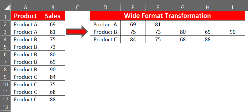
Suppose you have data that is stored in long format in Excel. You want to transpose it to wide format.
Example : Suppose you have data in columns A and B as shown in the table below : -
| A | B | |
|---|---|---|
| 1 | Product | Sales |
| 2 | Product A | 69 |
| 3 | Product A | 81 |
| 4 | Product B | 75 |
| 5 | Product B | 73 |
| 6 | Product B | 80 |
| 7 | Product B | 69 |
| 8 | Product B | 90 |
| 9 | Product C | 84 |
| 10 | Product C | 75 |
| 11 | Product C | 68 |
| 12 | Product C | 88 |
We want the output in wide format as shown in the image below. Please note that data in columns A and B can have any value (character or numeric).
Follow the steps below to transpose data from a vertical format to a horizontal one.
Step 1 : To pull unique values from Column A, type the following formula in cell D2.
=IFERROR(INDEX($A$2:$A$100, MATCH(0,COUNTIF($D1:D$1, $A$2:$A$100), 0)),"")
Press CTRL + SHIFT + ENTER to confirm this formula as it's an array formula. If this formula is entered correctly, you would see the formula inside the curly brackets {}.
Step 2 : To fetch values from column B, type the following formula in cell E2.
=IF(COLUMN(A1)<=COUNTIF($A$1:$A$100,"="&$D2),OFFSET(INDIRECT("$B"&MATCH($D2,$A$1:$A$100,0)),COLUMN(A1)-1,0),"")
This formula finds value of cell D2 in column A and gives back related values from column B. In other words, it is similar to a VLOOKUP function but can return multiple corresponding values from column B for a lookup value.
Step 3 : Select the formula in cell D2 and paste it down to the cells below. Similarly, select the formula in cell E2 and paste it to the right and down. Use Ctrl+R to paste to the right and Ctrl+D to paste down.

Deepanshu founded ListenData with a simple objective - Make analytics easy to understand and follow. He has over 10 years of experience in data science. During his tenure, he worked with global clients in various domains like Banking, Insurance, Private Equity, Telecom and HR.
The data in Column A must be numbers?
ReplyDeleteI tried text data and got wrong results
yes, it must definitely be numbers, in order
DeleteWe have another formula for extracting unique numbers
DeleteAlternatively you can copy on a different sheet and drop duplicates
The second COUNTIF should be a MATCH() instead. It should be:
ReplyDelete=IF(COLUMN(A1) <=COUNTIF($A$1:$A$100,"="&$D2),OFFSET(INDIRECT("$B"& MATCH($D2,$A$1:$A$100,0)),COLUMN(A1)-1,0),"")
Thank you so much it works
DeleteNot so useful IMHO because the resulting columns have the various stocks listed helter-skelter, for instance, column E has Stocks D, O, D, Q, P. Usually you'd want all the D's stacked, etc.
ReplyDeleteWhat if the table had more than two columns?
ReplyDeleteI have an excel sheet with four columns and more than 6000 rows. I have tried this formula and it only works for two columns and up to cell 100 across the two columns. How do I modify to suit my data?
ReplyDeleteUse the =Transpose(range) function.
ReplyDeleteThis is really useful. Can you please expain each formula. This will be helpful in applying this formula to larger data sheets.
ReplyDeleteThanks! This is a good way to solve those problems ;). I would like to understand how works every formula in the same post, however, Great article!! 10/10
ReplyDeleteThere is an easier way using matrix function
ReplyDelete