CARET Package Implementation in R

In R, there is a package called caret which stands for Classification And REgression Training. It makes predictive modeling easy. It can run most of the predive modeling techniques with cross-validation. It can also perform data slicing and pre-processing data modeling steps.

Loading required libraries
library(C50)
library(ROCR)
library(caret)
library(plyr)
Set Parallel Processing - Decrease computation time
install.packages("doMC")
library(doMC)
registerDoMC(cores = 5)
Splitting data into training and validation

The following code splits 60% of data into training and remaining into validation.
trainIndex <- createDataPartition(data[,1], p = .6, list = FALSE, times = 1)
dev <- data[ trainIndex,]
val  <- data[-trainIndex,]
In this code, a data.frame named "data" contains full dataset. The list = FALSE avoids returns the data as a list. This function also has an argument, times, that can create multiple splits at once; the data indices are returned in a list of integer vectors.

Similarly, createResample can be used to make simple bootstrap samples and createFolds can be used to generate balanced cross–validation groupings from a set of data.

Repeated K Fold Cross-Validation
cvCtrl <- trainControl(method = "repeatedcv", number =10, repeats =3, classProbs = TRUE)
Explanation : 
  1. repeatedcv : repeated K-fold cross-validation 
  2. number = 10 : 10-fold cross-validations
  3. repeats = 3 : three separate 10-fold cross-validations are used.
  4. classProbs = TRUE : It should be TRUE if metric = " ROC " is used in the train function. It can be skipped if metric = "Kappa" is used.
Note : Kappa measures accuracy.

There are two ways to tune an algorithm in the Caret R package :
  1. tuneLength =  It allows system to tune algorithm automatically. It indicates the number of different values to try for each tunning parameter. For example, mtry for randomForest. Suppose, tuneLength = 5, it means try 5 different mtry values and find the optimal mtry value based on these 5 values.
  2. tuneGrid =  It means user has to specify a tune grid manually. In the grid, each algorithm parameter can be specified as a vector of possible values. These vectors combine to define all the possible combinations to try. 
For example,  grid = expand.grid(.mtry= c(1:100))

grid = expand.grid(.interaction.depth = seq(1, 7, by = 2), .n.trees = seq(100, 1000, by = 50), .shrinkage = c(0.01, 0.1))

Example 1 : train with tuneGrid (Manual Grid)
grid <- expand.grid(.model = "tree", .trials = c(1:100), .winnow = FALSE)

set.seed(825)
tuned <- train(dev[, -1], dev[,1], method = "C5.0", metric = "ROC",
               tuneGrid = grid, trControl = cvCtrl)

Example 2 : train with tunelength (Automatic Grid)
set.seed(825)
tuned <- train(dev[, -1], dev[,1], method = "C5.0", metric = "ROC",
               tunelength = 10, trControl = cvCtrl)

Finding the Tuning Parameter for each of the algorithms

Visit this link - http://topepo.github.io/caret/modelList.html

Calculating the Variable Importance
varImp(tuned$finalModel , scale=FALSE)
plot(varImp(tuned$finalModel))
To get the area under the ROC curve for each predictor, the filterVarImp function can be used. The area under the ROC curve is computed for each class.
RocImp <- filterVarImp(x = dev[, -1], y = dev[,1])
RocImp
# Seeing result
tuned

# Seeing Parameter Tuning
trellis.par.set(caretTheme())
plot(tuned, metric = "ROC")

# Seeing final model result
print(tuned$finalModel)

#Summaries of C5.0 Model
summary(tuned$finalModel)

# variable Importance
C5imp(tuned$finalModel, metric="usage")

#Scoring
val1 = predict(tuned$finalModel, val[, -1], type = "prob")

Other Useful Functions
  1. nearZeroVar: a function to remove predictors that are sparse and highly unbalanced
  2. findCorrelation: a function to remove the optimal set of predictors to achieve low pair–wise correlations (Check out this link)
  3. preProcess: Variable selection using PCA 
  4. predictors: class for determining which predictors are included in the prediction equations (e.g. rpart, earth, lars models) (currently7 methods)
  5. confusionMatrix, sensitivity, specificity, posPredValue, negPredValue: classes for assessing classifier performance
Spread the Word!
Share

Difference between CHAID and CART

Classification and Regression Trees (CART)

Regression Tree : The outcome (dependent) variable is a continuous variable and predictor (independent) variables can be continuous or categorical variables (binary). It creates binary split.

Algorithm of Regression Tree:  Least-Squared Deviation or Least Absolute Deviation 

The impurity of a node is measured by the Least-Squared Deviation (LSD), which is simply the variance within the node.

Classification Tree : The outcome (dependent) variable is a categorical variable (binary) and predictor (independent) variables can be continuous or categorical variables (binary). It creates binary split.

Note : If the dependent variable has more than 2 categories, then C4.5 algorithm or conditional inference tree algorithm should be used.

Algorithm of Classification Tree: Gini Index

Gini Index measures impurity in node. It varies between 0 and (1-1/n) where n is the number of categories in a dependent variable.

Process :
  1. Rules based on variables' values are selected to get the best split to differentiate observations based on the dependent variable
  2. Once a rule is selected and splits a node into two, the same process is applied to each "child" node (i.e. it is a recursive procedure)
  3. Splitting stops when CART detects no further gain can be made, or some pre-set stopping rules are met. (Alternatively, the data are split as much as possible and then the tree is later pruned.

CHAID

CHAID stands for Chi-square Automated Interaction Detection.

The outcome (dependent) variable can be continuous and categorical. But, predictor (independent) variables are categorical variables only (can be more than 2 categories). It can create multiple splits (more than 2).

When independent variables are continuous, they need to be transformed into categorical variables (bins/groups) before using CHAID.

Algorithm : 

If dependent variable is categorical, Chi-Square test determines the best next split at each step.

If dependent variable is continuous, F test determines the best next split at each step.

Process : 

Cycle through the predictors to determine for each predictor the pair of (predictor) categories that is least significantly different with respect to the dependent variable; for classification problems (where the dependent variable is categorical as well), it will compute a Chi-square test (Pearson Chi-square); for regression problems (where the dependent variable is continuous), F tests. If the respective test for a given pair of predictor categories is not statistically significant as defined by an alpha-to-merge value, then it will merge the respective predictor categories and repeat this step (i.e., find the next pair of categories, which now may include previously merged categories). If the statistical significance for the respective pair of predictor categories is significant (less than the respective alpha-to-merge value), then (optionally) it will compute a Bonferroni adjusted p-value for the set of categories for the respective predictor.

Selecting the split variable. The next step is to choose the split the predictor variable with the smallest adjusted p-value, i.e., the predictor variable that will yield the most significant split; if the smallest (Bonferroni) adjusted p-value for any predictor is greater than some alpha-to-split value, then no further splits will be performed, and the respective node is a terminal node.

Continue this process until no further splits can be performed (given the alpha-to-merge and alpha-to-split values). (Source : Statsoft)

Comparison of CHAID and CART


How CHAID is better than CART ?

1. CHAID uses multiway splits by default (multiway splits means that the current node is splitted into more than two nodes). Whereas, CART does binary splits (each node is split into two daughter nodes) by default.
2. CHAID prevents overfitting problem. A node is only split if a significance criterion is fulfilled.
Spread the Word!
Share

Ensemble Learning : Boosting and Bagging

In this article, we will cover the concepts of bagging and boosting. It also includes how Stochastic Gradient Boosting works.

Ensemble learning

Ensemble learning is a machine learning concept in which idea is to train multiple models (learners) to solve the same problem.

The main advantages of Ensemble learning methods are :
  1. Reduced variance : Overcome overfitting problem. Low variance means model independent of training data. Results are less dependent on features of a single model and training set.
  2. Reduced bias : Overcome underfitting problem. Low bias means linear regression applied to linear data, second degree polynomial applied to quadratic data. Combination of multiple classifiers may produce more reliable classification than single classifier.

Bagging (Bootstrap Aggregating)

Generates m new training data sets.  Each new training data set picks a sample of observations with replacement (bootstrap sample) from original data set.  By sampling with replacement, some observations may be repeated in each new training data set. The m models are fitted using the above m bootstrap samples and combined by averaging the output (for regression) or voting (for classification).

Example :

Random forest is one of the most important bagging ensemble learning algorithm, In random forest, approx. 2/3rd of the total training data (63.2%) is used for growing each tree. And the remaining one-third of the cases (36.8%) are left out and not used in the construction of each tree. Each tree gives a classification, and we say the tree "votes" for that class. The forest chooses the classification having the most votes over all the trees in the forest. For a binary dependent variable, the vote will be YES or NO, count up the YES votes. This is the RF score and the percent YES votes received is the predicted probability. In regression case, it is average of dependent variable.

Uses of Bagging Algorithm
  1. It is designed to improve the stability and accuracy of machine learning algorithms used in statistical classification and regression.
  2. It also reduces variance and helps to avoid overfitting


Boosting Algorithm

Layman's Term : AdaBoost Algorithm

In this example, we focus on boosting algorithm, especially Adaboost algorithm.
  1. Start by creating a tree on training data, where each observation is assigned an equal weight.
  2. Then compute the predicted classification and weights are redetermined and assign greater weight to those observations that are difficult to classify and lower weights to those that are easy to classify. Weights for all observations must sum to 1.
  3. Second tree is grown on weighted data (weights are based on residuals or misclassification error). Idea is to improve prediction of first tree.
  4. Weights are redetermined and assign higher weights if it is classified incorrectly.
  5. New Model is now Tree 1 + Tree 2
  6. Compute residuals or classification error from this new 2-tree model (Tree1 + Tree2) and grow 3rd tree to predict revised residuals.
  7. Then subsequent trees help in classifying observations that are not well classified by preceding trees.
  8. The final prediction is a weighted sum of the predictions made by previous tree models. 
In this process, we have created many simple decision trees, where each tree is built for the prediction errors (classification error) of the previous tree.

Why Boosting works?

We weight misclassified observations in such a way that they get properly classified in future iterations.

Main Idea
  • Combine several simple decision trees (can be hundred or thousands)
  • Each tree complements the previous ones (Avoid redundancy)
  • Keep track of the errors of the previous trees
This technique is faced with a problem of overfitting

Stochastic Gradient Boosting Algorithm

To overcome problem of overfitting, stochastic gradient boosting comes into picture.

A general solution to the overfitting problem is to evaluate the quality of the fitted model by predicting observations in a test-sample of data that have not been used before to estimate the respective model(s). In Stochastic Gradient Boosting (GBM), a similar solution is implemented.

Let's first understand Gradient Descent!

What is Gradient Descent?

It tries to optimize the loss function by tuning different values of weights or coefficients to minimize the error. It is a method which comprises a vector of weights (or coefficients) where we calculate their partial derivative with respective to zero. The motive behind calculating their partial derivative is to find the local minima of the loss function (Residual Sum of Squares), which is convex in nature.

To train the model, we need to optimize a loss function. It is the function we need to minimize.

Loss Functions

Loss or Error Function for Classification

Minimizing Loss Function means maximising accuracy of the classifier.
Gradient Boosting minimize logistic regression's LogLoss (aka negative log-likelihood or bernoulli function)Bernoulli distribution is a special case of the binomial distribution with n=1. AdaBoost minimizes Exponential Loss function.

Log Loss or Bernoulli :  

LogLoss can be expressed in form of  
Logloss = [∑ y log(pᵢ) + (1-y) log(1 - pᵢ)] * -(1/N)
Here, Pi is logistic function. Refer the image below -
logistic function 

LogLoss = -(sum((actual*log(predicted)+(1-actual)*log(1-predicted)) / length(actual)
In this case, actual means 1 and predicted means predicted probability (It's same probability that is derived from model).

Important Points about LogLoss

The idea is to minimize the negative log-likelihood. It can also be read as maximizing log-likelihood.
The reason for taking the negative of the logarithm of the likelihood are as follows -It is because log(probability) will be negative so we take negative of log(p) to make it positive so that it would easy for comparison.

Loss function for Regression : Squared Error
(y - f(x))^2
It is called squared-loss function. y-f(x) : residual

Important Points :
  1. Residuals can be interpreted as negative gradients.
  2. For Classification, Gradient Descent Loss Function = Log-loss function.
  3. For Regression, Gradient Descent Loss Function = Squared loss function.

How Stochastic Gradient Boosting Works

  1. Simple tree is built on original target variable by taking only a randomly selected subsample of the dataset. It implements 'Stochastic' boosting techniqueParameter :  bag.fraction :  sampling rate (0.5). In this case, 0.5 implies only 50% of the data used at each iteration.
  2. The tree is built as small as two nodes and typically in the range of 4-8 nodes (Parameter:  interaction.depth : Nodes per tree)
  3. We score full training data using this tree model and compute the negative gradient (i.e. residual or classification error) for every record
  4. Make residual as a new target (dependent) variable
  5. Grow second tree to predict the residuals from first tree. Idea is to improve first tree.
  6. Each tree is weighted by a small weight prior to being used to compute the current prediction or score produced by the model.This means that the model prediction changes by very small amounts after a new tree is added to the model. It is to reduce the impact of each additional tree. The weighting factor is also called shrinkage or learning rate.
  7. We combine two trees by taking score for any record that come from the first tree and add to it the score that comes from the second tree. The second tree can therefore be thought of as correcting the predictions of the first tree. So a model from the end of a Gradient Boosting process is simply the sum of all the scores of all the trees that were built.
  8. Now, we have revised model with two trees. Third tree is grown on residuals from model consisting of first two tree. The whole process keeps on going.
  9. It yield models (i.e. additive weighted expansions of simple trees) that generalize well to new observations, i.e., exhibit good predictive validity.
Also, like in bagging, subsampling allows one to define an out-of-bag estimate of the prediction performance improvement by evaluating predictions on those observations which were not used in the building of the next base learner. Out-of-bag estimates help avoid the need for an independent validation dataset, but often underestimate actual performance improvement and the optimal number of iterations.

Important Point
Prediction in Gradient Boosting models are made not by combining voting of all the trees, but cumulative predictions of all the trees.

Difference between Bagging and Boosting
  1. In Boosting, each model is built on top of the previous ones. Whereas in bagging each model is built independently.
  2. The final boosting ensemble uses weighted majority vote while bagging uses a simple majority vote.
  3. Bagging is a method of reducing variance while boosting can reduce the variance and bias of the base classifier
  4. Boosting is better than bagging on non-noisy data
  5. Bagging is effective more often than boosting

R Packages for Boosting and Bagging
  1. gbm - The gbm package offers two versions of boosting for classification (gentle boost under logistic and exponential loss). In addition, it includes squared error, absolute error, Poisson and Cox type loss functions.
  2. ada - Performs discrete, real, and gentle boost under both exponential and logistic loss on a given data set.
  3. randomForest - Random Forest Package (Bagging)
Spread the Word!
Share

4 ways to find maximum value in a group with SAS

Suppose you have sales data. You wish to find maximum sales generated by a product ID.

data test;
input ID product $  Sale;
cards;
1 A 4.5
1 B 1
1 C 4.25
1 D 3
1 E  4.75
2 F 4.9
2 G  4.1
2 H 3
2 I 4
2 J  4.05
;
run;

Method I . 
proc sort data = test;
by ID descending sale;
run;

proc sort data = test nodupkey;
by ID;
run;

Method II. 

proc sort data = test;
by ID descending sale;
run;

data test1;
set test;
by ID;
If first.ID then output test1;
run;

Method III. 
proc sort data = test;
by ID;
run;

proc rank data=test out= test2(where=(sale_rank=1))  ties=low descending;
by ID;
var sale;
ranks sale_rank;
run;

Method IV. 
proc sql noprint;
create table t1 as
select * from test a inner join
(select ID, max(sale) as maxsale
from test
group by ID) b
on a.ID = b.ID and a.sale = b.maxsale;
quit;
Spread the Word!
Share

Conditional Mean Missing Imputation with SAS

Suppose you need to impute missing values with conditional mean in SAS.

proc standard data = test replace out= outdata;
by b;
var a;
run;
Spread the Word!
Share

Multiple Imputation with SAS

This tutorial explains multiple imputation and how it works. It also includes implementation of the algorithm with SAS and also challenges attached to it.

Multiple Imputation

Instead of filling in a single value for each missing value, multiple imputation (Rubin 1976, 1987) replaces each missing value with a set of plausible values that represent the uncertainty about the right value to impute. The multiply imputed data sets are then analyzed by using standard procedures for complete data and combining the results from these analyses. No matter which complete-data analysis is used, the process of combining results from different data sets is essentially the same. [Source : SAS Website]

This process draws a random sample of the missing values from its distribution. This process results in valid statistical inferences that properly reflect the uncertainty due to missing values—for example, confidence intervals with the correct probability coverage.

Multiple imputation inference involves three distinct phases:
  1. The missing data are filled in m times to generate m complete data sets.
  2. Perform regression or any other analysis on each of the m complete data sets.
  3. Average the values of the parameter estimates across the M samples to produce a single point estimate.
  4. Calculate the standard errors by averaging the standard errors of the M parameter estimates. Also calculate variance of the M parameter estimates across samples.

Objective of Multiple Imputation
The main goal of Multiple Imputation is to get robust estimates of your model. It means model is unbiased by missing data.

In SAS, Proc MI is used to replace missing values with multiple imputation.

Missing Data Patterns

1. Monotone : 

If a variable has missing data, all variables to the right of the missing data variable in a rectangular data array are also missing.


For example, If an observation has missing value in the third variable, monotonic missing is like o o m m m (all variables to the right has missing data), and one kind of non-monotonic missing can be o o m o m, where o indicates observed, m indicates missing.

2. Arbitrary:

Arbitrary missing data is a missing data pattern that has missingness spread among full data values (no observed missing data pattern).


I.  MCMC : Markov Chain Monte Carlo method (Default Method)

The MCMC method is used to impute missing values for a data set with an arbitrary missing pattern. This is the default method in PROC MI (METHOD=MCMC).

PROC MI data = mi_input_data seed=44853 nimpute=5 out=mi_output_data ;
multinormal method=mcmc;
var outcome age gender ethnicity BMI FBS heart_rate ;
run ;
PROC LOGISTIC data=mi_output_data outest=outreg covout;
class gender ;
model outcome= age gender age gender ethnicity BMI FBS heart_rate /covb ;
by _imputation_ ;ods output ParameterEstimates=mi_parms CovB=mi_covb;
run ;
PROC MIANALYZE  data = outreg;
modeleffects Intercept age gender ethnicity BMI FBS heart_rate ;
run ;

NIMPUTE = specifies the number of imputations. In this case, it is 5.

IMPUTATION : When this program runs it will produce a large new dataset with 5 * number of observations in a dataset. It will also include a variable called Imputation. For example, you have 150 observations in a dataset. The first 150 observations will have Imputation = 1, the next 150 have Imputation = 2, and so on.

PROC MIANALYZE : It performs the final analysis, which takes the results of the five logistic regressions and combines them.

Interpretation : We average across the five sets of coefficients, we average across the standard errors, and we take the variability of regression coefficients across the five sets of imputed data.


Important PROC MI Statements
  1. CLASS specifies the classification variables in the VAR statement
  2. MONOTONE specifies imputation methods for a data set with a monotone missing pattern
  3. VAR specifies the variables to be analyzed (both missing and non-missing)

II. Regression Imputation (Linear Regression)

proc mi data=Fish1 seed=13951639 out=outex3;
Class Length1
monotone reg(Length1 Length2)
var Length1 Length2 Length3;
run;

Note : Length1 and Length2 are variables to be imputed.

III. Imputing Nominal and Ordinal variables (Discriminant and Logistic Regression)

proc mi data=Fish seed=1305417 out=OutFish;
class Species;
logistic( Species= Length Height Width Height*Width/ details);
var Length Height Width Species;
run;

Ordinal and Binary : Logistic option
Non-Binary : Discrim option
Nominal and Binary : Discrim option

In the above code, Species is a variable on which missing data exists. Var statement includes list of both missing and non-missing variables to be used as predictors in the imputation models.

Example Code : Both Categorical and Continuous Data

proc mi data=Fish seed=1305417 out=OutFish;
class Species;
monotone reg(Height Width/ details)
logistic( Species= Length Height Width Height*Width/ details);
var Length Height Width Species;
run;
Spread the Word!
Share

Missing Value Imputation based on Clustering

The clustering based missing imputation assigns observations to clusters and fill in cluster means for missing observations.

Example 

Suppose the variable X1 is Cost and X2 is Salary. The non-missing cases have been clustered into three clusters.

Now you have a case with a value for Cost but not for Salary.

  • You determine which cluster's mean value is closest to the Cost value. 
  • Suppose this value of Cost is closest to the mean of the second cluster. 
  • To impute the missing value of Salary, you replace it with the mean value of  Salary for the second cluster.

proc fastclus data=training impute outiter outseed=seed out=training1 maxclusters=5;
var outcome survrate prognos amttreat gsi avoid intrus;
run;
Options in PROC FASTCLUS

  1. IMPUTE requests imputation of missing values after the final assignment of observations to clusters. 
  2. OUTITER outputs information from the iteration history to the OUTSEED= data set, including the cluster seeds at each iteration.
  3. OUTSEED= is another name for the MEAN= data set, provided because the data set can contain location estimates other than means.
  4. MAXCLUSTERS= specifies the maximum number of clusters permitted. If you omit the MAXCLUSTERS= option, a value of 100 is assumed.

PROC FASTCLUS is then used to replace the missing values from the validation data set with the cluster means from the training data set computed at the first iteration.
proc fastclus data=valid impute seed=seed(where=(_iter_=1)) replace=none maxclusters=5 out=validate1 maxiter=0;
var outcome survrate prognos amttreat gsi avoid intrus;
run;
SEED= specifies an input data set from which initial cluster seeds are to be selected.

REPLACE= specifies how seed replacement is performed. NONE suppresses the seed replacement.
Spread the Word!
Share

SAS: How to Fill Missing Values

In this article, we will explain how you can impute missing values using the PROC STDIZE procedure in SAS.

SAS: Fill Missing Values
Sample Dataset

Let's create two different sample datasets for training and validation for demonstration purposes.

data training;
  input v1 v2 v3;
  datalines;
10 20 30
. 25 35
5 . 25
20 30 .
;
run;

data validation;
  input v1 v2 v3;
  datalines;
15 18 20
15 . 25
. 21 30
10 30 .
;
run;

Replace Missing Values with Zero

The REPONLY option in PROC STDIZE procedure tells SAS to replace missing data and not standardize the data. You can specify the numeric value for replacing missing values in MISSING= option in PROC STDIZE. The following code replaces missing values in the variables (v1, v2, and v3) in the "training" dataset with zero (0) and then output the filled data to "training2".

PROC STDIZE DATA=TRAINING OUT=TRAINING2 MISSING=0 REPONLY;
VAR V1 V2 V3;
RUN;

Replace Missing Values with Mean

The following code replaces missing values in the variables (v1, v2, and v3) in the "training" dataset with the mean of non-missing values and then output the filled data to "training2". The "outstat=info" option saves statistics of the missing values to a dataset named "info."

proc stdize data=training out=training2 method=mean reponly outstat=info;
var v1 v2 v3;
run;
You can also replace mean with median as a method of imputing missing values.

Impute Missing Values in Validation Data Using Training Data

To fill missing values in the validation data based on values from the training data, you can use method=in(dataset) option in PROC STDIZE procedure.

proc stdize data=validation out=validation2 reponly method=in(info);
var v1 v2 v3;
run;

The resulting dataset "validation2" will contain the missing values in the validation dataset filled with mean values from the training dataset.

Spread the Word!
Share

SAS Macro : A Dynamic Loop

Suppose you need to pass a variable within a loop based on the input defined in a SAS macro using the %DO statement.

The following code defines a macro named "report" that calculates summary statistics using the PROC MEANS procedure for each variable specified in the var parameter and groups them by the variable specified in the "class" parameter. It then outputs the statistics to separate datasets. The names of the output datasets are dynamically generated based on the loop index.

%macro report (input=, var = , class=);
%let n=%sysfunc(countw(&var));
%do i=1 %to &n;
%let val = %scan(&var,&i);
proc means data = &input noprint nway;
class &class;
vars &val;
output out=out&i mean= median= / autoname;
run;
%end;
%mend;

options mprint;
%report(input= test, var = b c, class=a);

When you execute the above sas program, it generates the following output :

proc means data = &input noprint nway;
class a;
vars b;
output out=out1 mean= median= / autoname;
run;

proc means data = input noprint nway;
class a;
vars c;
output out=out2 mean= median= / autoname;
run;
Spread the Word!
Share

SAS : Brier Score for Model Calibration

The Brier score is an important measure of calibration i.e. the mean squared difference between the predicted probability and the actual outcome.
Lower the Brier score is for a set of predictions, the better the predictions are calibrated.
  1. If the predicted probability is 1 and it happens, then the Brier Score is 0, the best score achievable.
  2. If the predicted probability is 1 and it does not happen, then the Brier Score is 1, the worst score achievable.
  3. If the predicted probability is 0.8 and it happens, then the Brier Score is (0.8-1)^2 =0.04.
  4. If the predicted probability is 0.2 and it happens, then the Brier Score is (0.2-1)^2 =0.64.
  5. If the predicted probability is 0.5, then the Brier Score is (0.5-1)^2 =0.25, irregardless of whether it happens.
By specifying fitstat option in proc logistic, SAS returns Brier score and other fit statistics such as AUC, AIC, BIC etc.
proc logistic data=train;
model y(event="1") = entry/ outroc = rocstats;
score data=valid out=valpred fitstat;
run;
Spread the Word!
Share

SAS : Calculating the optimal predicted probability cutoff

There are three ways to calculate optimal probability cut-off :
  1. Youden's J Index
  2. Minimize Euclidean distance of sensitivity and specificity from the point (1,1)
  3. Profit Maximization / Cost Minimization

Youden's J index is used to select the optimal predicted probability cut-off. It is the maximum vertical distance between ROC curve and diagonal line. The idea is to maximize the difference between True Positive and False Positive.

Youden Index Formula
J = Sensitivity - (1 - Specificity )
Optimal probability cutoff is at where J is maximum.

Euclidean Distance Formula
D = Sqrt ((1-Sensitivity)^2 + (1-Specificity)^2)
Optimal probability cutoff is at where D is minimum.

SAS Code

proc logistic data = test descending;
model y = x1 x2 / outroc=rocstats;
run;

data check;
set rocstats;
_SPECIF_ = (1 - _1MSPEC_);
J = _SENSIT_ + _SPECIF_ - 1;
D= Sqrt((1-_SENSIT_)**2 + (1-_SPECIF_)**2);
run;

proc sql noprint;
create table cutoff as
select _PROB_ , J
from check
having J = max(J);
run;

proc sql noprint;
create table cutoff1 as
select _PROB_ , D
from check
having D = min(D);
run;
Spread the Word!
Share

SAS Macro : Determine the number of rows and variables in a dataset

Suppose you need to find out the number of rows and number of character and numeric variables in a data set.
data _null_;
if 0 then set correl nobs=n;
array nums _numeric_;
array chars _character_;
nvar = dim(nums);
cvar = dim(chars);
tvar= nvar + cvar;
call symput ('nrows',n);
call symput('numer',nvar);
call symput('chars',cvar);
call symput('totvar',tvar);
run;

%put &nrows;
%put &numer;
%put &chars;
%put &totvar;

In this program, correl is a data set.
Spread the Word!
Share

SAS Macro : Count number of variables assigned in a macro variable

Suppose you need to identify the number of variables user input in a macro variable.

Option I 
%macro nvars (ivars);
%let n=%sysfunc(countw(&ivars));
%put &n;
%mend;
%nvars (X1 X2 X3 X4);
Option II 
%macro nvars (ivars);

%let n=1;
%do %until ( %scan(&ivars,&n)= );
%let n=%EVAL(&n + 1);
%end;

%let n=%eval(&n-1);
%put &n;
%mend;

%nvars ( X1 X2 X3 X4);
Spread the Word!
Share

Detect Non-Linear and Non- Monotonic Relationship between Variables

In linear regression analysis, it's an important assumption that there should be a linear relationship between independent variable and dependent variable. Whereas, logistic regression assumes there should be a linear relationship between independent variable and logit function.

How to check non-linearity

Pearson correlation is a measure of linear relationship. The variables must be measured at interval scales. It is sensitive to outliers. If pearson correlation coefficient of a variable is close to 0, it means there is no linear relationship between variables.

Spearman's correlation is a measure of monotonic relationship. It can be used for ordinal variables. It is less sensitive to outliers. If spearman correlation coefficient of a variable is close to 0, it means there is no monotonic relationship between variables.

Hoeffding’s D correlation is a measure of linear, monotonic and non-monotonic relationship. It has values between –0.5 to 1. The signs of Hoeffding coefficient has no interpretation.
If a variable has a very low rank for Spearman (coefficient - close to 0) and a very high rank for Hoeffding indicates a non-monotonic relationship.
If a variable has a very low rank for Pearson (coefficient - close to 0) and a very high rank for Hoeffding indicates a non-linear relationship.

Criterion to eliminate irrelevant variables
If a variable has poor rank on both the spearman and hoeffding correlation metrics, it means the relationship between the variables is random.

SAS Macro to detect non-monotonic relationship
Spread the Word!
Share

SAS: Impute Missing Values

Suppose you have data consisting of 1000 variables and you need to impute missing values with mean/median. You can do it easily with PROC STDIZE.

proc stdize data= test out= result method=mean reponly;
var X1-X1000;
run;

By specifying the REPONLY option, the STDIZE procedure does not standardize the numeric variables; it replaces the missing values with the METHOD= statistic.

Other Useful METHOD= statistic options

  1. MEDIAN
  2. MIDRANGE
  3. IQR
  4. MAXABS : Maximum Absolute Value
  5. STD : Standard Deviation

If you want to replace missing values with 0 or any number
proc stdize data=develop1 reponly missing=0 out=imputed;
var mortdue value yoj derog delinq clage ninq clno debtinc;
run;

Note : You cannot use MISSING and METHOD options together.

Spread the Word!
Share

SAS : Proc Varclus Explained

The VARCLUS procedure is a useful SAS procedure for variable reduction. It is based on divisive clustering technique.
  1. All variables start in one cluster. Then, a principal components analysis is done on the variables in the cluster to determine whether the cluster should be split into two subsets of variables.
  2. If the second eigenvalue for the cluster is greater than the specified cutoff, then the inital cluster is split into two clusters. If the second eigenvalue is large, it means that at least two principal components account for a large amount of variation among the inputs.
  3. To determine which inputs are included in each cluster, the principal component scores are rotated obliquely to maximize the correlation within a cluster and minimize the correlation between clusters. 
  4. This process ends when the second eigenvalues of all current clusters fall below the cutoff.
If a cluster has only 1 variable in it, it means that this variable has only one principal component and hence, second eigenvalue of this variable is 0.
proc varclus data=imputed maxeigen=.7 short hi;
var Q1-Q5 VAR1-VAR20;
run;
The MAXEIGEN option specifies the largest permissible value of the second eigenvalue in each cluster (default value is 1)

The HI option specifies that the clusters at different levels maintain a hierarchical structure that prevents variables from transferring from one cluster to another after the split is made. In other words, variables cannot be reassigned to other clusters as they are assigned once in a cluster.

The SHORT option suppresses some of the output generated by PROC VARCLUS.

Important Points
  1. By default, maximum clusters is equal to the number of variables in the model. The MAXCLUSTERS option can be used to specify the largest number of clusters desired. It's better not to specify the option and let SAS decides the number of clusters.
  2. By default, PROC VARCLUS uses a non-hierarchical version of this algorithm, in which variables can also be reassigned to other clusters. The HI option is used to run hierarchical version.
  3. Larger eigenvalue thresholds result in fewer clusters, and smaller thresholds yield more clusters.
  4. Variables belonging to different clusters may be correlated as it is a type of oblique component analysis.

How to select best variables from each cluster

A best variable has a high correlation with its own cluster and has a low correlation with the other clusters.
A variable that has the lowest 1- R-squared ratio is likely to be a good representative for the cluster. It means maximum correlation with own cluster and minimum correlation with next cluster.
Why lowest 1 - R-squared ratio?

It is because when a variable has maximum correlation with own cluster and minimum correlation with next cluster. the 1- R**2 ratio will be minimum. See the formula below.


SAS Macro for Variable Selection

%macro varsel(input=, vars= , output =);
ods select none;
ods output clusterquality=summary
           rsquare=clusters;

proc varclus data=&input maxeigen=.7 short hi;
   var &vars;
run;
ods select all;

data _null_;
set summary;
call symput('nvar',compress(NumberOfClusters));
run;

data selvars;
set clusters (where = (NumberOfClusters=&nvar));
keep Cluster Variable RSquareRatio;
run;

data cv / view=cv;
retain dummy 1;
set selvars;
keep dummy cluster;
run;

data filled;
update cv(obs=0) cv;
by dummy;
set selvars(drop=cluster);
output;
drop dummy;
run;

proc sort data = filled;
by cluster RSquareRatio;
run;

data &output;
set filled (rename = (variable = Best_Variables));
if first.cluster then output;
by cluster;
run;

%mend;

%varsel(input= abc, vars= _numeric_ , output = rest);

Same Variable Selection Technique (Varlcus) in R
install.packages("Hmisc")
v = varclus(x, similarity="spear")
R Code : IV and Clustering
Spread the Word!
Share

Weight of Evidence (WOE) and Information Value (IV) Explained

In this article, we will cover the concept of Weight of Evidence (WOE) and Information Value (IV) and how they can be used to improve your predictive model along with the details of how to compute them using SAS, R and Python.

Logistic regression model is one of the most commonly used statistical technique for solving binary classification problem. It is an acceptable technique in almost all the domains. These two concepts - weight of evidence (WOE) and information value (IV) evolved from the same logistic regression technique. These two terms have been in existence in credit scoring world for more than 4-5 decades. They have been used as a benchmark to screen variables in the credit risk modeling projects such as probability of default. They help to explore data and screen variables. It is also used in marketing analytics project such as customer attrition model, campaign response model etc.

Table of Contents

What is Weight of Evidence?

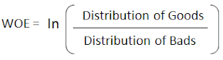
The Weight of Evidence (WOE) tells the predictive power of an independent variable in relation to the dependent variable. Since it evolved from credit scoring world, it is generally described as a measure of the separation of good and bad customers. "Bad Customers" refers to the customers who defaulted on a loan. and "Good Customers" refers to the customers who paid back loan.

Weight of Evidence
WOE Calculation
Distribution of Goods - % of Good Customers in a particular group
Distribution of Bads - % of Bad Customers in a particular group
ln - Natural Log
Positive WOE means Distribution of Goods > Distribution of Bads
Negative WOE means Distribution of Goods < Distribution of Bads
Hint : Log of a number > 1 means positive value. If less than 1, it means negative value.
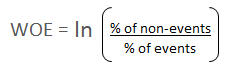
Many people do not understand the terms goods/bads as they are from different background than the credit risk. It's good to understand the concept of WOE in terms of events and non-events. It is calculated by taking the natural logarithm (log to base e) of division of % of non-events and % of events.
WOE = In(% of non-events ➗ % of events)
WOE Formula
Weight of Evidence Formula

How to calculate Weight of Evidence?

Follow the steps below to calculate Weight of Evidence

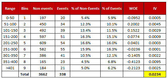
  1. For a continuous variable, split data into 10 parts (or lesser depending on the distribution).
  2. Calculate the number of events and non-events in each group (bin)
  3. Calculate the % of events and % of non-events in each group.
  4. Calculate WOE by taking natural log of division of % of non-events and % of events
Note : For a categorical variable, you do not need to split the data (Ignore Step 1 and follow the remaining steps)
Weight of Evidence and Information Value
Weight of Evidence and Information Value Calculation


Download : Excel Template for WOE and IV

Terminologies related to WOE

1. Fine Classing
Create 10/20 bins/groups for a continuous independent variable and then calculates WOE and IV of the variable
2. Coarse Classing
Combine adjacent categories with similar WOE scores

Usage of WOE

Weight of Evidence (WOE) helps to transform a continuous independent variable into a set of groups or bins based on similarity of dependent variable distribution i.e. number of events and non-events.

For continuous independent variables : First, create bins (categories / groups) for a continuous independent variable and then combine categories with similar WOE values and replace categories with WOE values. Use WOE values rather than input values in your model.
data age1;
set age;
if age = . then WOE_age = 0.34615;
if age >= 10 then WOE_age = -0.03012;
if age >= 20 then WOE_age = 0.07689;
run;

proc logistic data=age1 descending;
model y = WOE_age;
run;
For categorical independent variables : Combine categories with similar WOE and then create new categories of an independent variable with continuous WOE values. In other words, use WOE values rather than raw categories in your model. The transformed variable will be a continuous variable with WOE values. It is same as any continuous variable.

Why combine categories with similar WOE?

It is because the categories with similar WOE have almost same proportion of events and non-events. In other words, the behavior of both the categories is same.
Rules related to WOE
  1. Each category (bin) should have at least 5% of the observations.
  2. Each category (bin) should be non-zero for both non-events and events.
  3. The WOE should be distinct for each category. Similar groups should be aggregated.
  4. The WOE should be monotonic, i.e. either growing or decreasing with the groupings.
  5. Missing values are binned separately.

Number of Bins (Groups)
In general, 10 or 20 bins are taken. Ideally, each bin should contain at least 5% cases. The number of bins determines the amount of smoothing - the fewer bins, the more smoothing. If someone asks you ' "why not to form 1000 bins?" The answer is the fewer bins capture important patterns in the data, while leaving out noise. Bins with less than 5% cases might not be a true picture of the data distribution and might lead to model instability.

Handle Zero Event/ Non-Event
If a particular bin contains no event or non-event, you can use the formula below to ignore missing WOE. We are adding 0.5 to the number of events and non-events in a group.

AdjustedWOE = ln (((Number of non-events in a group + 0.5) / Number of non-events)) / ((Number of events in a group + 0.5) / Number of events))

How to check correct binning with WOE

1. The WOE should be monotonic i.e. either growing or decreasing with the bins. You can plot WOE values and check linearity on the graph.
2. Perform the WOE transformation after binning. Next, we run logistic regression with 1 independent variable having WOE values. If the slope is not 1 or the intercept is not ln(% of non-events / % of events) then the binning algorithm is not good. [Source : Article]

Benefits of Weight of Evidence

Here are some benefits of Weight of Evidence and how it can be used to improve your predictive model.

  1. It can treat outliers. Suppose you have a continuous variable such as annual salary and extreme values are more than 500 million dollars. These values would be grouped to a class of (let's say 250-500 million dollars). Later, instead of using the raw values, we would be using WOE scores of each classes.
  2. It can handle missing values as missing values can be binned separately.
  3. Since WOE Transformation handles categorical variable so there is no need for dummy variables.
  4. WoE transformation helps you to build strict linear relationship with log odds. Otherwise it is not easy to accomplish linear relationship using other transformation methods such as log, square-root etc. In short, if you would not use WOE transformation, you may have to try out several transformation methods to achieve this.

What is Information Value?

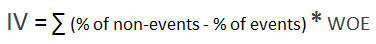
Information value (IV) is one of the most useful technique to select important variables in a predictive model. It helps to rank variables on the basis of their importance. The IV is calculated using the following formula :

IV = ∑ (% of non-events - % of events) * WOE
Information Value Formula

Rules related to Information Value

Information Value Variable Predictiveness
Less than 0.02 Not useful for prediction
0.02 to 0.1 Weak predictive Power
0.1 to 0.3 Medium predictive Power
0.3 to 0.5 Strong predictive Power
>0.5 Suspicious Predictive Power

According to Siddiqi (2006), by convention the values of the IV statistic in credit scoring can be interpreted as follows.

If the IV statistic is:
  1. Less than 0.02, then the predictor is not useful for modeling (separating the Goods from the Bads)
  2. 0.02 to 0.1, then the predictor has only a weak relationship to the Goods/Bads odds ratio
  3. 0.1 to 0.3, then the predictor has a medium strength relationship to the Goods/Bads odds ratio
  4. 0.3 to 0.5, then the predictor has a strong relationship to the Goods/Bads odds ratio.
  5. > 0.5, suspicious relationship (Check once)
Important Points
  1. Information value increases as bins / groups increases for an independent variable. Be careful when there are more than 20 bins as some bins may have a very few number of events and non-events.
  2. Information value is not an optimal feature (variable) selection method when you are building a classification model other than binary logistic regression (for eg. random forest or SVM) as conditional log odds (which we predict in a logistic regression model) is highly related to the calculation of weight of evidence. In other words, it's designed mainly for binary logistic regression model. Also think this way - Random forest can detect non-linear relationship very well so selecting variables via Information Value and using them in random forest model might not produce the most accurate and robust predictive model.
How to calculate WOE and IV for Continuous Dependent Variable
WOE and IV for Continuous Dependent Variable

Python, SAS and R Code : WOE and IV

R Code

Follow the steps below to calculate Weight of Evidence and Information Value in R

Step 1 : Install and Load Package
First you need to install 'Information' package and later you need to load the package in R.
install.packages("Information")
library(Information)
Step 2 : Import your data
#Read Data
mydata <- read.csv("https://stats.idre.ucla.edu/stat/data/binary.csv")
Step 3 : Summarise Data
In this dataset, we have four variables and 400 observations. The variable admit is a binary target or dependent variable.
summary(mydata)
     admit            gre           gpa            rank     
 Min.   :0.000   Min.   :220   Min.   :2.26   Min.   :1.00  
 1st Qu.:0.000   1st Qu.:520   1st Qu.:3.13   1st Qu.:2.00  
 Median :0.000   Median :580   Median :3.40   Median :2.00  
 Mean   :0.318   Mean   :588   Mean   :3.39   Mean   :2.48  
 3rd Qu.:1.000   3rd Qu.:660   3rd Qu.:3.67   3rd Qu.:3.00  
 Max.   :1.000   Max.   :800   Max.   :4.00   Max.   :4.00 

Step 4 : Data Preparation
Make sure your independent categorical variables are stored as factor in R. You can do it by using the following method -
mydata$rank <- factor(mydata$rank)
Important Note : The binary dependent variable has to be numeric before running IV and WOE as per this package. Do not make it factor.
Step 5 : Compute Information Value and WOE
In the first parameter, you need to define your data frame followed by your target variable. In the bins= parameter, you need to specify the number of groups you want to create it for WOE and IV.
IV <- create_infotables(data=mydata, y="admit", bins=10, parallel=FALSE)
It takes all the variables except dependent variable as predictors from a dataset and run IV on them.

This function supports parallel computing. If you want to run you code in parallel computing mode, you can run the following code.
IV <- create_infotables(data=mydata, y="admit", bins=10, parallel=TRUE)
You can add ncore= parameter to mention the number of cores to be used for parallel processing.

Information Value in R 
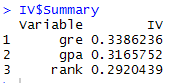
In IV list, the list Summary contains IV values of all the independent variables.
IV_Value = data.frame(IV$Summary)
Information Value Scores
To get WOE table for variable gre, you need to call Tables list from IV list.
print(IV$Tables$gre, row.names=FALSE)
       gre  N Percent     WOE    IV
 [220,420] 38  0.0950 -1.3748 0.128
 [440,480] 40  0.1000 -0.0820 0.129
 [500,500] 21  0.0525 -1.4860 0.209
 [520,540] 51  0.1275  0.2440 0.217
 [560,560] 24  0.0600 -0.3333 0.223
 [580,600] 52  0.1300 -0.1376 0.225
 [620,640] 51  0.1275  0.0721 0.226
 [660,660] 24  0.0600  0.7653 0.264
 [680,720] 53  0.1325  0.0150 0.265
 [740,800] 46  0.1150  0.7653 0.339
To save it in a data frame, you can run the command below-
gre = data.frame(IV$Tables$gre)
Plot WOE Scores
To see trend of WOE variables, you can plot them by using plot_infotables function.
plot_infotables(IV, "gre")
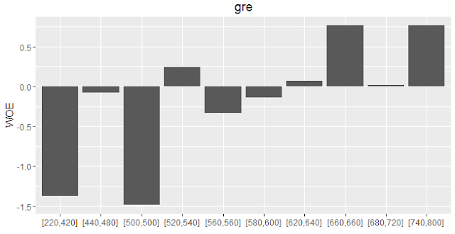
WOE Plot

To generate multiple charts on one page, you can run the following command -
plot_infotables(IV, IV$Summary$Variable[1:3], same_scale=FALSE)
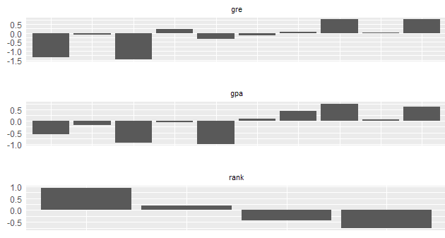
Calculate WOE and IV in R
MultiPlot WOE

Important Point
It is important to note here the number of bins for 'rank' variable. Since it is a categorical variable, the number of bins would be according to unique values of the factor variable. The parameter bins=10 does not work for a factor variable.

Python Code

Here are the steps on how to calculate Weight of Evidence and Information Value in Python:

Load Required Python Packages
You can import packages by using import module in Python. The 'as' keyword is used for alias. Instead of using the package name, we can use alias to call any function from the package.
#Load Required Packages
import pandas as pd
import numpy as np
By using read_csv( ) function, we can read CSV file into Python.
#Read Data
mydata = pd.read_csv("https://stats.idre.ucla.edu/stat/data/binary.csv")
Python Function to calculate Information Value and WOE
def iv_woe(data, target, bins=10, show_woe=False):
    
    #Empty Dataframe
    newDF,woeDF = pd.DataFrame(), pd.DataFrame()
    
    #Extract Column Names
    cols = data.columns
    
    #Run WOE and IV on all the independent variables
    for ivars in cols[~cols.isin([target])]:
        if (data[ivars].dtype.kind in 'bifc') and (len(np.unique(data[ivars]))>10):
            binned_x = pd.qcut(data[ivars], bins,  duplicates='drop')
            d0 = pd.DataFrame({'x': binned_x, 'y': data[target]})
        else:
            d0 = pd.DataFrame({'x': data[ivars], 'y': data[target]})
        d0 = d0.astype({"x": str})
        d = d0.groupby("x", as_index=False, dropna=False).agg({"y": ["count", "sum"]})
        d.columns = ['Cutoff', 'N', 'Events']
        d['% of Events'] = np.maximum(d['Events'], 0.5) / d['Events'].sum()
        d['Non-Events'] = d['N'] - d['Events']
        d['% of Non-Events'] = np.maximum(d['Non-Events'], 0.5) / d['Non-Events'].sum()
        d['WoE'] = np.log(d['% of Non-Events']/d['% of Events'])
        d['IV'] = d['WoE'] * (d['% of Non-Events']-d['% of Events'])
        d.insert(loc=0, column='Variable', value=ivars)
        print("Information value of " + ivars + " is " + str(round(d['IV'].sum(),6)))
        temp =pd.DataFrame({"Variable" : [ivars], "IV" : [d['IV'].sum()]}, columns = ["Variable", "IV"])
        newDF=pd.concat([newDF,temp], axis=0)
        woeDF=pd.concat([woeDF,d], axis=0)

        #Show WOE Table
        if show_woe == True:
            print(d)
    return newDF, woeDF
In this user-defined function, there are 4 parameters user needs to mention.
  1. data means data frame in which dependent and independent variable(s) are stored.
  2. target refers to name of dependent variable.
  3. bins refers to number of bins or intervals. By default, it is 10.
  4. show_woe = True means you want to print the WOE calculation Table. By default, it is False
How to run Function
It returns two dataframes named iv and woe which contains Information value and WOE of all the variables.
iv, woe = iv_woe(data = mydata, target = 'admit', bins=10, show_woe = True)
print(iv)
print(woe)
Important Points related to Python Script
  1. Dependent variable specified in target parameter must be binary. 1 refers to event. 0 refers to non-event.
  2. All numeric variables having no. of unique values less than or equal to 10 are considered as a categorical variable. You can change the cutoff in the code len(np.unique(data[ivars]))>10
  3. IV score generated from python code won't match with the score derived from R Package as pandas function qcut( ) does not include lowest value of each bucket. It DOES NOT make any difference in terms of interpretation or decision making based on WOE and IV result.

SAS Code

Here is the SAS program that demonstrates how to calculate the Weight of Evidence and Information Value:

/* IMPORT CSV File from URL */
FILENAME PROBLY TEMP;
PROC HTTP
 URL="https://stats.idre.ucla.edu/stat/data/binary.csv"
 METHOD="GET"
 OUT=PROBLY;
RUN;

OPTIONS VALIDVARNAME=ANY;
PROC IMPORT
  FILE=PROBLY
  OUT=WORK.MYDATA REPLACE
  DBMS=CSV;
RUN;


PROC HPBIN DATA=WORK.MYDATA QUANTILE NUMBIN=10;
INPUT GRE GPA;
ODS OUTPUT MAPPING = BINNING;
RUN;

PROC HPBIN DATA=WORK.MYDATA WOE BINS_META=BINNING;
TARGET ADMIT/LEVEL=BINARY ORDER=DESC;
ODS OUTPUT INFOVALUE = IV WOE = WOE_TABLE;
RUN;
  1. NUMBIN= refers to number of bins you want to create in WOE calculation.
  2. INPUT refers to all the continuous independent variables
  3. TARGET Specify target or dependent variable against this statement
  4. ORDER=DESC tells SAS that 1 refers to event in your target variable
Output values of WOE and IV using above SAS and Python code would match exactly. R package Information implemented slightly different algorithm and cutoff technique so its returned values may differ with the values from Python and SAS code but difference is not huge and interpretation remains same.
Related Tutorials
Spread the Word!
Share

Checking Assumptions of Multiple Regression with SAS

This article explains how to check the assumptions of multiple regression and the solutions to violations of assumptions.

Download the dataset (Source : UCLA)

SAS Code : Reading downloaded file into SAS
/* Read data from a folder where the file is stored*/
libname reg "C:\Users\Deepanshu Bhalla\Downloads";

/* Checking the number of observations, number of variables in a data set*/
proc contents data = reg.crime varnum;
run;
Read Statistical Properties of OLS Coefficient Estimators

Checking Assumptions of Multiple Regression with SAS

1. Detecting Outlier

I. Box Plot Method

If a value is higher than the 1.5*IQR above the upper quartile (Q3), the value will be considered as outlier. Similarly, if a value is lower than the 1.5*IQR below the lower quartile (Q1), the value will be considered as outlier. In SAS, PLOTS options in PROC UNIVARIATE tells SAS to generate Box Plot graph.


II. Studentized Residuals Method

Studentized Residuals : Meaning

Before jumping into studentized residuals, we need to understand the meaning of residuals. 

Residuals is the difference between the observed value and the predicted value.
Standardized Residuals is the residuals divided by the standard error of estimate.
Studentized Residuals is the residuals divided by the standard error of the residual with that case deleted.
If absolute value of studentized residual is greater than 3, the observation is considered as an outlier.
SAS Code

/* Studentized residuals - Check Outliers*/
ods graphics on;
proc reg data=reg.crime;
model crime=pctmetro poverty single / stb clb;
output out=stdres p= predict r = resid rstudent=r h=lev cookd=cookd dffits=dffit;
run;
quit;
ods graphics off;

/* Print only those observations having absolute value of studentized residual greater than 3*/
proc print data= stdres;
var r crime pctmetro poverty single;
where abs(r)>=3;
run;

III. Cook's D Method

Higher the Cook's D is, the more influential the point is.
If the Cook's D value is greater than 4/(number of observations), the value is considered as an outlier.
SAS Code

proc print data=stdres;
where cookd > (4/51);
var cd crime pctmetro poverty single;
run;


Consequences of Outliers
Outliers can affect the estimates of the independent variables

Treatment of Outlier

1. Percentile capping based on distribution of a variable

It means replacing extreme values with the largest/smallest non-extreme observation.

In layman's terms, capping at the 1st and 99th percentile means values that are less than the value at 1st percentile are replaced by the value at 1st percentile, and values that are greater than the value at 99th percentile are replaced by the value at 99th percentile.


2. Compare Models with or without Outliers
Smaller the RMSE, Better the Model.
The RMSE is the square root of the variance of the residuals. It indicates the absolute fit of the model to the data–how close the observed data points are to the model’s predicted values. Whereas R-squared is a relative measure of fit, RMSE is an absolute measure of fit.  Lower values of RMSE indicate better fit. 

2. Linear Relationship between Dependent and Independent Variables

I. Scatter plot of independent variable vs. dependent variable

ods graphics on;
proc reg data=reg.crime;
model crime=pctmetro poverty single / partial;
run;
quit;
ods graphics off;

II . Run correlation between dependent variable and independent variables

There should be a moderate and SIGNIFICANT correlation score between dependent variable and independent variable.

proc corr data=reg.crime;
var pctmetro poverty single;
with crime;
run;

Check out : SAS Macro for detecting non-linear relationship


Consequences of Non-Linear Relationship

If the assumption of linearity is violated, the linear regression model will return incorrect (biased) estimates. In short, the coefficients as well as R-square will be underestimated.


Treatment of Non linear Relationship

1. When the error variance appears to be constant (Homoscedasticity), only X needs be transformed to linearize the relationship. Transform independent variable to Log10(X), Inverse(X), Square root(X), Square(X), Exp(X), 1/X, Exp(-X).

2. When the error variance does not appear constant it may be necessary to transform Y or both X and Y. Run Box-Cox Transformations for Dependent Variable


3. Errors (Residuals) should be normally distributed

The Shapiro-Wilk W test can be used to check normality assumption. In this case, we set null hypothesis that residual is normally distributed.
If the p-value is greater than .05, it means we cannot reject the null hypothesis that residual is normally distributed.
SAS Code

proc reg data=reg.crime;
model crime=pctmetro poverty single / stb clb;
output out=stdres p= predict r = resid;
run;

proc univariate data=stdres normal;
var resid;
run;

Consequences of Non-Normality of Errors

Many common tests of null hypotheses on regression results require normality. So if the residuals are not normal, then you cannot perform these hypothesis tests.

Treatment of Non Normality

Transform the DEPENDENT variable. Try log, square root and reciprocal transformations.
Run Box-Cox Transformations for Dependent Variable


4. Homoscedasticity

There should be homogeneity of variance of the residuals. In other words, the variance of residuals are approximately equal for all predicted dependent variable values.

Another way of thinking of this is that the variability in values for your independent variables is the same at all values of the dependent variable.

I. Plot Residuals by Predicted values

proc reg data= reg.crime;
model crime = poverty single;
plot r.*p.;
run;
quit;


II. White, Pagan and Lagrange multiplier (LM) Test

The White test tests the null hypothesis that the variance of the residuals is homogenous (equal). We use the / spec option on the model statement to obtain the White test.
If the p-value of white test is greater than .05, the homogenity of variance of residual has been met.
With PROC REG ( No CLASS statement , No Pagan Test)
proc reg data= reg.crime;
model crime = poverty single / SPEC;
run;
Note : P-value greater than .05 indicates homoscedasticity.
 With PROC AUTOREG (LM Test, CLASS statement for categorical variables)
proc autoreg data=reg.crime;
model crime = pctmetro poverty single / archtest;
output out=r r=yresid;
run;
Note : Check P-value of Q statistics and LM tests. P-value greater than .05 indicates homoscedasticity.

With PROC MODEL (White and Pagan Test , No CLASS statement for categorical variables)
proc model data= reg.crime;
parms a1 b1 b2;
crime = a1 + b1*poverty + b2*single;
fit crime / white pagan=(1 poverty single)
out=resid1 outresid;
run;
quit; 
If the p-value of white test and Breusch-Pagan test is greater than .05, the homogenity of variance of residual has been met.

Consequences of Heteroscedasticity
  1. The regression prediction remains unbiased and consistent but inefficient. It is inefficient because the estimators are no longer the Best Linear Unbiased Estimators (BLUE). 
  2. The hypothesis tests (t-test and F-test) are no longer valid.

Treatment of Heteroscedasticity

Testing and Correcting Heteroscedasticity

5. Multicollinearity

Mutlicollinearity  means there is a high correlation between independent variables. The linear regression model MUST NOT be faced with problem of multicollinearity.

VIF (Variance Inflation Factor)

It measures how much the variance of an estimated regression coefficient is increased because of collinearity.
Interpretation : If the variance inflation factor of a predictor variable were 9 (Sqrt(9) = 3) this means that the standard error for the coefficient of that predictor variable is 3 times as large as it would be if that predictor variable were uncorrelated with the other predictor variables.
If VIF is greater than 5, there is a multicollinearity problem in the model.
proc reg data = reg.crime;
model crime = poverty single / vif;
run;

Consequences of Multicollinearity

Multicollinearity inflates the standard errors, making it impossible to determine the relative
importance of the predictors. In other words, the coefficients will be unreliable. Note that multicollinearity does not affect the efficiency of the estimators – they remain BLUE (Best Linear Unbiased Estimators).

Treatment of Multicollinearity

1. Run PROC VARCLUS with HI option (Principal Component Analysis). A variable that has the lowest 1-R2 ratio is likely to be a good representative for the cluster.

2. Use centering: which is subtracting the mean from the predictor values before generating the square term. The resulting centered data may well display considerably lower multicollinearity.

For example : Weight and Weight2 are faced with problem of multicollinearity.

First Step : Center_Weight = Weight - mean(Weight)
Second Step : Center_Weight2 = Center_Weight ^2


6. Independence of error terms - No Autocorrelation

It states that the errors associated with one observation are not correlated with the errors of any other observation. It is a problem when you use time series data. Suppose you have collected data from labors in eight different districts. It is likely that the labors within each district will tend to be more like one another that labors from different districts, that is, their errors are not independent.

proc reg data = reg.crime;
model crime = poverty single / dw;
run;

PROC REG tests for first-order autocorrelations using the Durbin-Watson coefficient (DW). The null hypothesis is no autocorrelation.
A DW value between 1.5 and 2.5 confirms the absence of  first-order autocorrelation. If DW value less than 1.5, it indicates positive autocorrelation. If DW value greater than 2.5, it indicates negative autocorrelation
Autocorrelation inflates significance results of coefficients by underestimating the standard errors of the coefficients. Hypothesis testing will therefore lead to incorrect conclusions.

Another alternative test : Lagrange Multiplier Test 

It can be used for more than one order of auto correlation. It consists of several steps. First, regress Y on Xs to get residuals. Compute lag value of residuals up to pth order. Replace missing values for lagged residuals with zeros. Rerun regression model including lagged residual variable as an independent variable.
proc autoreg data = reg.crime;
model crime = poverty single / dwprob godfrey;
run;
Consequences of Autocorrelation
Autocorrelation inflates t-statistics by underestimating the standard errors of the coefficients. Hypothesis testing will therefore lead to incorrect conclusions. Estimators no longer have minimum variance but they will remain unbiased.

Treatment of Autocorrelation

1. Add lagged transforms (lag value) of the dependent variable


2. Use PROC AUTOREG 

It is advisable to build auto-regressive model with PROC AUTOREG for time series data.

Related Posts : 
  1. Linear Regression Model with PROC GLMSELECT
  2. Homoscedasticity Simplified with SAS
  3. Scoring Linear Regression Model with SAS

Important Point 1 : Box Cox Transformation of Dependent Variable can solve problem of non-linearity, non-normality of error and heteroscedasticity.
Run Box-Cox Transformations for Dependent Variable

Important Point 2 : RMSE for Training vs Test Sample

The RMSE for your training and your test sets should be very similar if you have built a good model. If the RMSE for the test set is much higher than that of the training set, it is likely that you've badly over fit the data, i.e. you've created a model that tests well in sample, but has little predictive value when tested out of sample.

Important Point 3 : Transformation Rules

Check out this link

The specific transformation used depends on the extent of the deviation from normality.

1. If the distribution differs moderately from normality, a square root transformation is often the best.
2. A log transformation is usually best if the data are more substantially non-normal.
3. An inverse transformation should be tried for severely non-normal data.
4. If nothing can be done to "normalize" the variable, then you might want to dichotomize (2 categories) the variable.
Spread the Word!
Share
Next → ← Prev