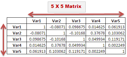
This article explains how to compute a correlation matrix using an excel formula.
What is Correlation matrix?
It is simply defined as the measure of the relationship between two or more variables. Coefficients have a range of -1 to 1; -1 is the perfect negative correlation while +1 is the perfect positive correlation. It is also called multiple correlation coefficient. The post below explains how to calculate multiple correlation coefficient in Excel.
Excel Formula to calculate Correlation Matrix
=CORREL(OFFSET(firstvariable_range,,ROWS($1:1)-1),OFFSET(firstvariable_range,,COLUMNS($A:A)-1))
For example, you have a 5 X 5 matrix and data for variables are entered in cells B3:F50 so paste this formula in cell J4
=CORREL(OFFSET($B$3:$B$50,,ROWS($1:1)-1),OFFSET($B$3:$B$50,,COLUMNS($A:A)-1))
In this case, firstvariable_range is B3:B50.
Download the workbook used in this example so you can copy and practice the formula.
How it works :
Let's take data for 5 variables and try to figure out the correlation between them.1. CORREL Function
Usage : It returns the correlation coefficient between two variables.
Syntax : = CORREL ( first variable_range, second variable_range )
For variable 1 and variable 2, the syntax would be =CORREL(B3:B50, C3:C50)
2. OFFSET Function
Usage : It returns a reference to a range that is a given number of rows and columns from a given reference Syntax : = OFFSET (reference range, number of rows up or down, number of columns to the left or right)
For example, = OFFSET($B$3:$B$50,,1) means one column to the right of B3:C50 i.e. C3:C50
3. ROWS / COLUMNS Function
Usage : It returns the number of rows or columns in a range. Syntax : = ROWS ( range ) For example, = ROWS ($1:2) returns 2.OR = COLUMNS ($A:B) returns 2
4. Dynamic CORREL Function
For variable 2 and variable 3,
=CORREL(OFFSET($B$3:$B$50,,ROWS($1:2)-1),OFFSET($B$3:$B$50,,COLUMNS($A:C)-1))i. ROWS($1:2) returns 2. Hence, ROWS($1:2)-1 returns 1
ii. OFFSET($B$3:$B$50,,ROWS($1:2)-1) returns reference of range C3:C50 i.e. data set for variable 2
iii. COLUMNS($A:C) returns 3. Hence, COLUMNS($A:C)-1 returns 2
iv. OFFSET($B$3:$B$50,,COLUMNS($A:C)-1) returns reference of variable 3

How to use it
Paste the formula below to N rows x N columns. In 5 X 5 matrix , paste down to 5 rows and right to 5 columns.
=CORREL(OFFSET($B$3:$B$50,,ROWS($1:1)-1),OFFSET($B$3:$B$50,,COLUMNS($A:A)-1))


Awesome, this saved me tons of time! Thank you for the step-by-step instructions.
ReplyDeleteThanks a lot!!
ReplyDeleteTHANK YOU VERY MUCH HELPED A LOT
ReplyDeleteThank you very helpful
ReplyDeleteThat's fantastic !!! Thank you so much !!!!
ReplyDeletecould you please write us the mathematical equation used to calculate the cross correlation coefficient.
ReplyDelete