This tutorial covers how to find out the maximum value based on a single or multiple criteria in Excel.
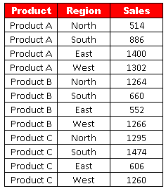
Suppose you have data for products, sales and regions.You are asked to find out the maximum sales generated by Product B. The data is shown in the image below.

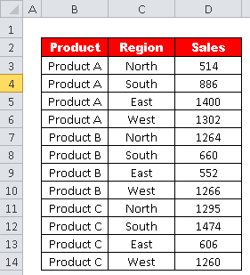
Assuming you have data in range B3:D14. (See the image below)

To calculate the maximum sales generated by Product B.
The values for the product are in cells B3:B14, and the values for sales are in cells D3:D14.
=MAX(IF(B3:B14="Product B",D3:D14))
Since the above formula is an array formula, press CTRL SHIFT ENTER to confirm it instead of simply pressing ENTER key.
After pressing CTRL SHIFT ENTER, the formula will be surrounded by curly braces and look like :
{=MAX(IF(B3:B14="Product B",D3:D14))}
IF(B3:B14="Product B", D3:D14): This is the conditional part of the formula. It checks each cell in the range B3:B14, and if the cell contains the text "Product B", it returns the corresponding value from the range D3:D14. Otherwise, it returnsFALSEor an empty cell.MAX(...): This function calculates the maximum value from the array produced by theIFfunction. It ignoresFALSEvalues and empty cells, focusing only on the numeric values.
How to Find the Maximum Value in Excel with Multiple Criteria
To calculate the maximum sales generated by Product B in East region .

=MAX(IF((B3:B14="Product B")*(C3:C14="East"),D3:D14))
Since the above formula is an array formula, press CTRL SHIFT ENTER to confirm it.
After pressing CTRL SHIFT ENTER, the formula will be surrounded by curly braces and look like :
{=MAX(IF((B3:B14="Product B")*(C3:C14="East"),D3:D14))}
B3:B14="Product B": This part checks each cell in the range B3:B14 to see if it contains the text "Product B". It returns an array of TRUE and FALSE values, where TRUE represents cells that meet the condition, and FALSE represents cells that don't.C3:C14="East": This part checks each cell in the range C3:C14 to see if it contains the text "East". It also returns an array of TRUE and FALSE values based on the condition.(B3:B14="Product B")*(C3:C14="East"): Here, both the arrays from steps 1 and 2 are combined using the * (asterisk) operator. This operation results in a new array that contains TRUE only for the rows where both conditions are met (i.e., where "Product B" is in column B and "East" is in column C).IF((B3:B14="Product B")*(C3:C14="East"),D3:D14): This is the conditional part of the formula. It uses the array from step 3 to filter the values in the range D3:D14. If the corresponding element in the array is TRUE, it includes the value from the range D3:D14. Otherwise, it returns FALSE or an empty cell.MAX(...): This function calculates the maximum value from the array produced by the IF function. It ignores FALSE values and empty cells, focusing only on the numeric values that satisfy the given conditions.


Share Share Tweet