This tutorial explains the VLOOKUP function in layman's language and how to use it in Excel, along with examples.
VLOOKUP: Introduction
The Vlookup function looks for a value in the leftmost column of a table and then returns a value in the same row from a column you specify.
Syntax of VLOOKUP
The syntax for Vlookup function is as follows :
VLOOKUP(lookup_value, table_array, col_index_num ,range_lookup)
VLOOKUP (value to be found, table reference, pull a matching value from the Kth column of the table , exact match / closest match)
- lookup_value - It is the value to be found in the first column of the table.
- table_array - It is a table of text, numbers or logical values. Table_array can be a cell reference or a range name.
- col_index_num - It is the column number in table_array from which the matching value should be returned.
- range_lookup - 1 (TRUE) - Find the closest match in first column sorted in ascending order. 0 (FALSE) - Find an exact match.
Example
Suppose you have data for students' names and their classes and sections. You want to find the class name for a student in the data table.
Download the workbook used in the examples shown below and practice what you learn.The data is shown in the image below :

=VLOOKUP(B12, $B$3:$E$8, 3, 0)The detailed explanation is shown in the image below :

In this case, Excel will search for the value in B12 within the range B3:E8. If it finds an exact match, it will return the value from column D. In the formula, 3 refers to the third column of the specified range B3:E8 which is column D.
Limitation of VLOOKUP
To make VLOOKUP work, you need to have a lookup value in the first column of the table. If your look up value is not placed in the first column of the table, it will return #N/A error.


Look up value must be in the leftmost column of a table
Advanced Vlookup Function
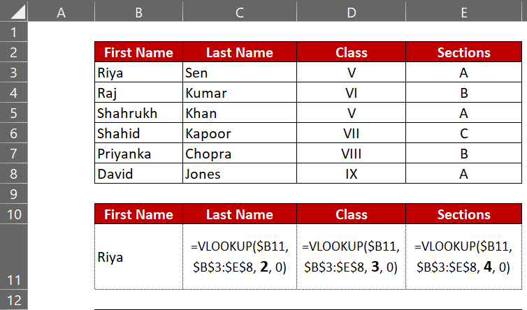
Suppose you want to do a dynamic column lookup based on the value in cell B11. Manually you need to change the formula in each cell (C11 through E11) to update the third parameter of Vlookup formula (col_index_num). Look at the image below.
Use the COLUMN function to increment column index number automatically by 1
=VLOOKUP($B11, $B$3:$E$8, COLUMN(B1), 0)How COLUMN function works?
It returns the column number of a cell reference.
For example, the formula =COLUMN(B1) returns 2, because column B is the second column.

After applying the formula in cell C11, paste the formula to the right (Select the cells C11 through E11 and press CTRL + R).
As shown in the image below, you can change the column from which you want to extract data by copying the formula to the right and the VLOOKUP will adjust accordingly.

Dynamic Vlookup Function
Suppose columns are not ordered in the table the way you want values to be returned.

Since the column index numbers are not in any proper order, we cannot use COLUMN function.
Instead we can use MATCH function to return the column index number.
=VLOOKUP($B11, $B$3:$E$8, MATCH(C10,$B$2:$E$2,0),0)
In this formula, we are using VLOOKUP with the MATCH function to dynamically select a column based on the value in cell C10 and pull data from the specified column in the range $B$3:$E$8.
How MATCH function works?The MATCH function returns the relative position of an item in an array that matches a specified value.
= MATCH(value to be found, range of cells being searched, match type)


After applying the formula in cell C11, paste the formula to the right (Select the cells C11 through E11 and press CTRL + R).= MATCH (C10, $B$2:$E2,0) evaluates to :
= MATCH("Last Name", ("First Name","Last Name","Class","Sections"), Find the closest match)
Result : It returns 2 as "Last Name" is placed second in list.
Download the workbook


Can you please explain how to find duplicate value in two different sheets using Vlookup and IFERROR . It will be of great help . And congratulation for such a wonderful site on Excel, SAS and analytics all together .
ReplyDeletevery helpful
ReplyDeleteHey Its really helpful to understand VlOOKUP. Thank you !
ReplyDeleteI have one doubt, In the Section how column works ? You have mention "Select Cells C11 through C13 and then press CTRL+R " but i think it should be "Select Cells C11 through E13 and then press CTRL+R". But on doing that, The counter value increases but "Look up value" changes and hence it shows N/A. And to fix that we need to manually change to the look up Value. Can you please make this understand ?
It should be cell C11 through E11 and then Press CTRL R. I have corrected it in the article. You can fix the reference of the cell column so that lookup value does not change automatically. For example, cell reference of lookup value is B11 so you should use $B11 in the first parameter of VLOOKUP (Mind the $ Sign before B). Hope it helps!
DeleteExcellent
ReplyDeleteVery useful and dimple explanation.
ReplyDeleteHi bro...Want to build VBA code for a user defined NthVlookup function which can provide me the vlookup value for nth occurence...
ReplyDelete