Difference between Adjusted R-squared and R-squared

In this tutorial, we will explain the difference between r-squared and adjusted r-squared. We will cover both the theory behind them and how to calculate them in Python, R and SAS.

---

R-squared (R²)

It measures the proportion of the variation in your dependent variable explained by all of your independent variables in the model. It assumes that every independent variable in the model helps to explain variation in the dependent variable. In reality, some independent variables (predictors) don't help to explain dependent (target) variable. In other words, some variables do not contribute in predicting target variable.

Mathematically, R-squared is calculated by dividing sum of squares of residuals (SSres) by total sum of squares (SStot) and then subtract it from 1. In this case, SStot measures total variation. SSreg measures explained variation and SSres measures unexplained variation.

As SSres + SSreg = SStot, R² = Explained variation / Total Variation

R-squared Equation

R-Squared is also called coefficient of determination. It lies between 0% and 100%. A r-squared value of 100% means the model explains all the variation of the target variable. And a value of 0% measures zero predictive power of the model. Higher R-squared value, better the model.

Adjusted R-Squared

It measures the proportion of variation explained by only those independent variables that really help in explaining the dependent variable. It penalizes you for adding independent variables that do not help in predicting the dependent variable in regression analysis.

Adjusted R-Squared can be calculated mathematically in terms of sum of squares. The only difference between R-square and Adjusted R-square equation is degree of freedom.

Adjusted R-Squared Equation

In the above equation, dft is the degrees of freedom n– 1 of the estimate of the population variance of the dependent variable, and dfe is the degrees of freedom n – p – 1 of the estimate of the underlying population error variance.

Adjusted R-squared value can be calculated based on value of r-squared, number of independent variables (predictors), total sample size.

Adjusted R-Squared Equation 2

Difference between R-square and Adjusted R-square

Here are the differences between R-square and Adjusted R-square:

1. Every time you add a independent variable to a model, the R-squared increases, even if the independent variable is insignificant. It never declines. Whereas Adjusted R-squared increases only when independent variable is significant and affects dependent variable.
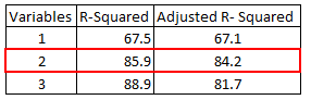
   In the table below, adjusted r-squared is maximum when we included two variables. It declines when third variable is added. Whereas r-squared increases when we included third variable. It means third variable is insignificant to the model.
   
2. Adjusted r-squared can be negative when r-squared is close to zero.
3. Adjusted r-squared value always be less than or equal to r-squared value.

Which is better?

Adjusted R-square should be used to compare models with different numbers of independent variables. Adjusted R-square should be used while selecting important predictors (independent variables) for the regression model.

Understand Adjusted R-squared with Example

Suppose you want to find out the relationship between the impact of advertising expenditure (X1) and the price of the product (X2) on the sales (Y).

Sales = β0 + β1 * Advertising + β2 * Price

Here β0 is intercept, β1 refers to slope/coefficient for advertising expenditure and β2 is coefficient/slope for the price of the product.

Let's say you run the linear regression model and the R-squared value came out 0.8 which means that 80% of the variation in sales can be explained by the advertising expenditure and the price of the product. Whereas the adjusted R-squared value would be lower than the R-squared value.

How to calculate R-Squared and Adjusted R-Squared

In this section, we will provide step-by-step instructions for calculating R-Squared and Adjusted R-Squared in Python, R, and SAS.

R : R-Squared and Adjusted R-Squared

Here is the R syntax for calculating R-Squared and Adjusted R-Squared.

Suppose you have actual and predicted dependent variable values. In the script below, we have created a sample of these values. In this example, y refers to the observed dependent variable and yhat refers to the predicted dependent variable.

y = c(21, 21, 22.8, 21.4, 18.7, 18.1, 14.3, 24.4, 22.8, 19.2)
yhat = c(21.5, 21.14, 26.1, 20.2, 17.5, 19.7, 14.9, 22.5, 25.1, 18)
R.squared = 1 - sum((y-yhat)^2)/sum((y-mean(y))^2)
print(R.squared)  

Final Result : R-Squared = 0.6410828

Let's assume you have three independent variables in this case.

n = 10
p = 3
adj.r.squared = 1 - (1 - R.squared) * ((n - 1)/(n-p-1))
print(adj.r.squared)  

In this case, adjusted r-squared value is 0.4616242 assuming we have 3 predictors and 10 observations.

Python : R-Squared and Adjusted R-Squared

Here is the Python code for calculating R-Squared and Adjusted R-Squared.

import numpy as np
y = np.array([21, 21, 22.8, 21.4, 18.7, 18.1, 14.3, 24.4, 22.8, 19.2])
yhat = np.array([21.5, 21.14, 26.1, 20.2, 17.5, 19.7, 14.9, 22.5, 25.1, 18])
R2 = 1 - np.sum((yhat - y)**2) / np.sum((y - np.mean(y))**2)
R2
n=y.shape[0]
p=3
adj_rsquared = 1 - (1 - R2) * ((n - 1)/(n-p-1))
adj_rsquared

In the code above, we are calculating R-squared value using the formula: 1 - (sum of squared residuals / sum of squared total variation). The squared residuals are obtained by subtracting the predicted values (yhat) from the observed values (y), then we square the differences, and sum them up. The squared total variation is obtained by subtracting the mean of the observed values (np.mean(y)) from each observed value, then we square the differences, and sum them up. Finally, the R-squared value is calculated by subtracting the ratio of squared residuals to squared total variation from 1

Adjusted R-squared value is calculated using the formula: 1 - (1 - R-squared) * ((n - 1)/(n - p - 1)). Here, n represents the number of observations, and p represents the number of predictors (independent variables) in the regression model.

SAS : R-Squared and Adjusted R-Squared

Below is the SAS program for calculating R-Squared and Adjusted R-Squared.

data temp;
input y yhat;
cards;
21 21.5
21 21.14
22.8 26.1
21.4 20.2
18.7 17.5
18.1 19.7
14.3 14.9
24.4 22.5
22.8 25.1
19.2 18
;
run;

 data out2;
  set temp ;
   d=y-yhat;
   absd=abs(d);
   d2 = d**2;
  run;

/* Residual Sum of Square */
proc means data = out2 ;
var d2;
output out=rss sum=;
run;

data _null_;
set rss;
call symputx ('rss', d2);
run;

%put &RSS.;

/* Total Sum of Square */
proc means data = temp ;
var y;
output out=avg_y mean=avg_y;
run;

data _null_;
set avg_y;
call symputx ('avgy', avg_y);
run;

%put &avgy.;

data out22;
set temp ;
diff = y - &avgy.;
diff2= diff**2;
run;

proc means data = out22 ;
var diff2;
output out=TSS sum=;
run;

data _null_;
set TSS;
call symputx ('TSS', diff2);
run;

/* Calculate the R2 */ 
%LET rsq = %SYSEVALF(1-&RSS./&TSS);
%put &RSQ;

/* Calculate the Adj R2 */
%LET N = 10;
%LET P = 3;
%let AdjRsqrd= %SYSEVALF(1 -((1-&rsq)*(&N-1)/(&N-&P-1)));
%PUT &AdjRsqrd;  

We have created a new dataset named out2 from the temp dataset. It calculates the differences between the actual (y) and predicted (yhat) values and stores them in the variable d. The absolute differences are stored in the variable absd. The squared differences are stored in the variable d2. proc means procedure was used to calculate the sum of squared differences ("d2") in the "out2" dataset.

The proc means procedure is used again to calculate the mean of y and store it in the variable avg_y. Then the differences between each actual value and the mean are calculated and squared, resulting in the variable diff2. Finally, we used the proc means procedure one more time to calculate the sum of squared differences diff2 in the out22 dataset, and the result (TSS) is stored in the dataset named TSS.

Related Posts

Statistics Tutorials : Top 50 Statistics Tutorials

Spread the Word!
Share Share Tweet

About Author:

Deepanshu founded ListenData with a simple objective - Make analytics easy to understand and follow. He has over 10 years of experience in data science. During his tenure, he worked with global clients in various domains like Banking, Insurance, Private Equity, Telecom and HR.

While I love having friends who agree, I only learn from those who don't
Let's Get Connected Email LinkedIn