This tutorial includes a step-by-step guide on running random forest in R. It provides an explanation of random forest in simple terms and how it works. You will also learn about training and validating the random forest model, along with details of the parameters used in the random forest R package.
What is Random Forest?
Random forest is a way of averaging multiple deep decision trees, trained on different parts of the same training set, with the goal of overcoming over-fitting problem of individual decision tree.
In other words, random forests are an ensemble learning method for classification and regression that operate by constructing a lot of decision trees at training time and outputting the class that is the mode of the classes output by individual trees.
Explaining your training data instead of finding patterns that generalize is what overfitting is. In other words, your model learns the training data by heart instead of learning the patterns which prevent it from being able to generalized to the test data. It means your model fits well to training dataset but fails to the validation dataset.
 |
| Random Forest Explained with R |
Decision Tree vs. Random Forest
Decision tree is encountered with over-fitting problem and ignorance of a variable in case of small sample size and large p-value. Whereas random forest is a type of recursive partitioning method particularly well-suited to small sample size and large p-value problems.
Random forest comes at the expense of a some loss of interpretability, but generally greatly boosts the performance of the final model.
Random Forest is one of the most widely used machine learning algorithm for classification. It can also be used for regression model (i.e. continuous target variable) but it mainly performs well on classification model (i.e. categorical target variable). It has become a lethal weapon of modern data scientists to refine the predictive model. The best part of the algorithm is that there are a very few assumptions attached to it so data preparation is less challenging and results to time saving. It's listed as a top algorithm (with ensembling) in Kaggle Competitions.
Can Random Forest be used both for Continuous and Categorical Target Variable?
Yes, it can be used for both continuous and categorical target (dependent) variable. In random forest/decision tree, classification model refers to factor/categorical dependent variable and regression model refers to numeric or continuous dependent variable.
How random forest works
Each tree is grown as follows:1. Random Record Selection : Each tree is trained on roughly 2/3rd of the total training data (exactly 63.2%) . Cases are drawn at random with replacement from the original data. This sample will be the training set for growing the tree.
2. Random Variable Selection : Some predictor variables (say, m) are selected at random out of all the predictor variables and the best split on these m is used to split the node.
By default, m is square root of the total number of all predictors for classification. For regression, m is the total number of all predictors divided by 3.The value of m is held constant during the forest growing.
Note : In a standard tree, each split is created after examining every variable and picking the best split from all the variables.
3. For each tree, using the leftover (36.8%) data, calculate the misclassification rate - out of bag (OOB) error rate. Aggregate error from all trees to determine overall OOB error rate for the classification. If we grow 200 trees then on average a record will be OOB for about .37*200=74 trees.
4. Each tree gives a classification on leftover data (OOB), and we say the tree "votes" for that class. The forest chooses the classification having the most votes over all the trees in the forest. For a binary dependent variable, the vote will be YES or NO, count up the YES votes. This is the RF score and the percent YES votes received is the predicted probability. In regression case, it is average of dependent variable.
For example, suppose we fit 500 trees, and a case is out-of-bag in 200 of them:
- 160 trees votes class 1
- 40 trees votes class 2
In this case, RF score is class1. Probability for that case would be 0.8 which is 160/200. Similarly, it would be an average of target variable for regression problem.
 |
| Out of Bag Predictions |
Average OOB prediction for the entire forest is calculated by taking row mean of OOB prediction of trees. See the result below -
 |
| Average OOB prediction |
Important Point
It is because each tree is grown on a bootstrap sample and we grow a large number of trees in a random forest, such that each observation appears in the OOB sample for a good number of trees. Hence, out of bag predictions can be provided for all cases.
What is random in Random Forest?
'Random' refers to mainly two process - 1. random observations to grow each tree and 2. random variables selected for splitting at each node. See the detailed explanation in the previous section.Important Point :
Random Forest does not require split sampling method to assess accuracy of the model. It performs internal validation as 2-3rd of available training data is used to grow each tree and the remaining one-third portion of training data always used to calculate out-of bag error to assess model performance.Pruning
In random forest, each tree is fully grown and not pruned. In other words, it is recommended not to prune while growing trees for random forest.
The best split is chosen based on Gini Impurity or Information Gain methods.
Preparing Data for Random Forest
1. Imbalance Data setA data set is class-imbalanced if one class contains significantly more samples than the other. In other words, non-events have very large number of records than events in dependent variable.
In such cases, it is challenging to create an appropriate testing and training data sets, given that most classifiers are built with the assumption that the test data is drawn from the same distribution as the training data.
Presenting imbalanced data to a classifier will produce undesirable results such as a much lower performance on the testing than on the training data. To deal with this problem, you can do undersampling of non-events.
Undersampling
It means down-sizing the non-events by removing observations at random until the dataset is balanced.2. Random forest is affected by multicollinearity but not by outlier problem.
3. Impute missing values within random forest as proximity matrix as a measure
Terminologies related to random forest
1. Bagging (Bootstrap Aggregating)Generates m new training data sets. Each new training data set picks a sample of observations with replacement (bootstrap sample) from original data set. By sampling with replacement, some observations may be repeated in each new training data set. The m models are fitted using the above m bootstrap samples and combined by averaging the output (for regression) or voting (for classification).
2. Out-of-Bag Error (Misclassification Rate)
Out-of-Bag is equivalent to validation or test data. In random forests, there is no need for a separate test set to validate result. It is estimated internally, during the run, as follows:
As the forest is built on training data , each tree is tested on the 1/3rd of the samples (36.8%) not used in building that tree (similar to validation data set). This is the out of bag error estimate - an internal error estimate of a random forest as it is being constructed.
3. Bootstrap Sample
It is a random with replacement sampling method.
Example : Suppose we have a bowl of 100 unique numbers from 0 to 99. We want to select a random sample of numbers from the bowl. If we put the number back in the bowl, it may be selected more than once. In this process, we are sampling randomly with replacement.
4. Proximity (Similarity)
Random Forest defines proximity between two observations :
- Initialize proximities to zeroes
- For any given tree, apply the tree to all cases
- If case i and case j both end up in the same node, increase proximity prox(ij) between i and j by one
- Accumulate over all trees in RF and normalize by twice the number of trees in RF
Proximity matrix is used for the following cases :
- Missing value imputation
- Outlier detection
Shortcomings of Random Forest
- Random Forests aren't good at generalizing cases with completely new data. For example, if I tell you that one ice-cream costs $1, 2 ice-creams cost $2, and 3 ice-creams cost $3, how much do 10 ice-creams cost? A linear regression can easily figure this out, while a Random Forest has no way of finding the answer.
- Random forests are biased towards the categorical variable having multiple levels (categories). It is because feature selection based on impurity reduction is biased towards preferring variables with more categories so variable selection (importance) is not accurate for this type of data.
The forest error rate depends on two things:
1. The correlation between any two trees in the forest. Increasing the correlation increases the forest error rate.
2. The strength of each individual tree in the forest. A tree with a low error rate is a strong classifier. Increasing the strength of the individual trees decreases the forest error rate.
Reducing mtry ( Number of random variables used in each tree) reduces both the correlation and the strength. Increasing it increases both. Somewhere in between is an "optimal" range of mtry - usually quite wide. Using the oob error rate a value of mtry in the range can quickly be found. This is the only adjustable parameter to which random forests is somewhat sensitive.
How to fine tune random forest
Two parameters are important in the random forest algorithm:- Number of trees used in the forest (ntree ) and
- Number of random variables used in each tree (mtry ).
First set the mtry to the default value (sqrt of total number of all predictors) and search for the optimal ntree value. To find the number of trees that correspond to a stable classifier, we build random forest with different ntree values (100, 200, 300….,1,000). We build 10 RF classifiers for each ntree value, record the OOB error rate and see the number of trees where the out of bag error rate stabilizes and reach minimum.
Find the optimal mtry
There are two ways to find the optimal mtry :
- Apply a similar procedure such that random forest is run 10 times. The optimal number of predictors selected for split is selected for which out of bag error rate stabilizes and reach minimum.
- Experiment with including the (square root of total number of all predictors), (half of this square root value), and (twice of the square root value). And check which mtry returns maximum Area under curve. Thus, for 1000 predictors the number of predictors to select for each node would be 16, 32, and 64 predictors.
How to use Random Forest to select the important features?
Random forest can be used to rank the importance of variables in a regression or classification problem.Interpretation : MeanDecreaseAccuracy table represents how much removing each variable reduces the accuracy of the model.Calculation : How Variable Importance works
- For each tree grown in a random forest, calculate number of votes for the correct class in out-of-bag data.
- Now perform random permutation of a predictor's values (let's say variable-k) in the oob data and then check the number of votes for correct class. By "random permutation of a predictor's values", it means changing the order of values (shuffling).
- Subtract the number of votes for the correct class in the variable-k-permuted data from the number of votes for the correct class in the original oob data.
- The average of this number over all trees in the forest is the raw importance score for variable k. The score is normalized by taking the standard deviation.
- Variables having large values for this score are ranked as more important. It is because if building a current model without original values of a variable gives worse prediction, it means the variable is important.
How to calculate Random Forest in R?
To calculate a Random Forest in R, follow the steps below:
Dataset Description : It's a German Credit Data consisting of 21 variables and 1000 records. The dependent or target variable is Creditability which explains whether a loan should be granted to a customer based on his/her profiles. You can download the file by clicking on this link and then right click >> Save As.Step I : Data Preparation
mydata= read.csv("https://raw.githubusercontent.com/deepanshu88/Datasets/master/UploadedFiles/german_credit.csv")
# Check types of variables
str(mydata)
'data.frame': 1000 obs. of  21 variables:
 $ Creditability                    : int  1 1 1 1 1 1 1 1 1 1 ...
 $ Account.Balance                  : int  1 1 2 1 1 1 1 1 4 2 ...
 $ Duration.of.Credit..month.       : int  18 9 12 12 12 10 8 6 18 24 ...
 $ Payment.Status.of.Previous.Credit: int  4 4 2 4 4 4 4 4 4 2 ...
 $ Purpose                          : int  2 0 9 0 0 0 0 0 3 3 ...
 $ Credit.Amount                    : int  1049 2799 841 2122 2171 2241 3398 1361 1098 3758 ...
 $ Value.Savings.Stocks             : int  1 1 2 1 1 1 1 1 1 3 ...
 $ Length.of.current.employment     : int  2 3 4 3 3 2 4 2 1 1 ...
 $ Instalment.per.cent              : int  4 2 2 3 4 1 1 2 4 1 ...
 $ Sex...Marital.Status             : int  2 3 2 3 3 3 3 3 2 2 ...
 $ Guarantors                       : int  1 1 1 1 1 1 1 1 1 1 ...
 $ Duration.in.Current.address      : int  4 2 4 2 4 3 4 4 4 4 ...
 $ Most.valuable.available.asset    : int  2 1 1 1 2 1 1 1 3 4 ...
 $ Age..years.                      : int  21 36 23 39 38 48 39 40 65 23 ...
 $ Concurrent.Credits               : int  3 3 3 3 1 3 3 3 3 3 ...
 $ Type.of.apartment                : int  1 1 1 1 2 1 2 2 2 1 ...
 $ No.of.Credits.at.this.Bank       : int  1 2 1 2 2 2 2 1 2 1 ...
 $ Occupation                       : int  3 3 2 2 2 2 2 2 1 1 ...
 $ No.of.dependents                 : int  1 2 1 2 1 2 1 2 1 1 ...
 $ Telephone                        : int  1 1 1 1 1 1 1 1 1 1 ...
 $ Foreign.Worker                   : int  1 1 1 2 2 2 2 2 1 1 ...
# Check number of rows and columns
dim(mydata)
# Make dependent variable as a factor (categorical)
mydata$Creditability = as.factor(mydata$Creditability)
Step II : Run the random forest model
library(randomForest)
set.seed(71)
rf <-randomForest(Creditability~.,data=mydata, ntree=500)
print(rf)
Note : If a dependent variable is a factor, classification is assumed, otherwise regression is assumed. If omitted, randomForest will run in unsupervised mode.
Type of random forest: classification
Number of trees: 500
No. of variables tried at each split: 4
        OOB estimate of  error rate: 23.1%
Confusion matrix:
    0   1 class.error
0 131 169  0.56333333
1  62 638  0.08857143
In this case, the number of variables tried at each split is based on the following formula. -1 is used as dataset contains dependent variable as well.
floor(sqrt(ncol(mydata) - 1))The number of variables selected at each split is denoted by mtry in randomforest function.
Step III : Find the optimal mtry value
Select mtry value with minimum out of bag(OOB) error.
mtry <- tuneRF(mydata[-1],mydata$Creditability, ntreeTry=500,
               stepFactor=1.5,improve=0.01, trace=TRUE, plot=TRUE)
best.m <- mtry[mtry[, 2] == min(mtry[, 2]), 1]
print(mtry)
print(best.m)
      mtry OOBError
3.OOB    3    0.241
4.OOB    4    0.233
6.OOB    6    0.236
In this case, mtry = 4 is the best mtry as it has least OOB error. mtry = 4 was also used as default mtry.
Parameters in tuneRF function
- The stepFactor specifies at each iteration, mtry is inflated (or deflated) by this value
- The improve specifies the (relative) improvement in OOB error must be by this much for the search to continue
- The trace specifies whether to print the progress of the search
- The plot specifies whether to plot the OOB error as function of mtry
Build model again using best mtry value.
set.seed(71)
rf <-randomForest(Creditability~.,data=mydata, mtry=best.m, importance=TRUE,ntree=500)
print(rf)
#Evaluate variable importance
importance(rf)
varImpPlot(rf)
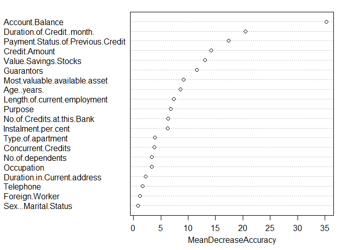 |
| Variable Importance |
Higher the value of mean decrease accuracy or mean decrease gini score , higher the importance of the variable in the model. In the plot shown above, Account Balance is most important variable.
- Mean Decrease Accuracy - How much the model accuracy decreases if we drop that variable.
- Mean Decrease Gini - Measure of variable importance based on the Gini impurity index used for the calculation of splits in trees.
pred1=predict(rf,type = "prob")
library(ROCR)
perf = prediction(pred1[,2], mydata$Creditability)
# 1. Area under curve
auc = performance(perf, "auc")
auc
# 2. True Positive and Negative Rate
pred3 = performance(perf, "tpr","fpr")
# 3. Plot the ROC curve
plot(pred3,main="ROC Curve for Random Forest",col=2,lwd=2)
abline(a=0,b=1,lwd=2,lty=2,col="gray")
 |
| ROC Curve |

Deepanshu founded ListenData with a simple objective - Make analytics easy to understand and follow. He has over 10 years of experience in data science. During his tenure, he worked with global clients in various domains like Banking, Insurance, Private Equity, Telecom and HR.
Great post - can you explain a bit about how the predicted probabilities are generated and what they represent in a more theoretical sense. I'm using randomForest but getting lots of 1.00 probabilities on my test set (bunching of probabilities) which is actually hurting me as i want to use them the filter out non relevant records in an unbiased fashion for further downstream work. I'm finding that logistic regression has a lot less of this going on. I'm combining the models to try get best of both. But as we usually think a probability of 1.00 can not exist, it's got me thinking about how to interpret probabilities from the RF model. Struggling to find a clear overview anywhere (will spend more time looking later).
ReplyDeleteAnyway nice post - adding this blog to my list :)
Very informative - thank you. I'm having trouble going 1 step deeper and actually interpreting the output from the importance(model) command. Applied, to the iris data set, the output looks like this:
ReplyDeletesetosa versicolor virginica MeanDecreaseAccuracy MeanDecreaseGini
Sepal.Length 1.277324 1.632586 1.758101 1.2233029 9.173648
Sepal.Width 1.007943 0.252736 1.014141 0.6293145 2.472105
Petal.Length 3.685513 4.434083 4.133621 2.5139980 41.284869
Petal.Width 3.896375 4.421567 4.385642 2.5371353 46.323415
Can you please help me understand what the numbers in the first 3 columns are - for example, the number 1.277324 in Row 1/Col 1 (sepal.width & Setosa).
I know Setosa is one of 3 classes and width is a feature, but, can't figure out what 1.277324 refers to.
Thank you!
hi, can you please explain the chart which is produced by plotting a RF model using plot function
ReplyDeleteLovely post. Everything at one place in a very simple language. I really enjoyed reading the article even late night.
ReplyDeleteKeep writing. I am looking forward to read other your posts too.
Thank you!
Hi, your post is very great!
ReplyDeleteI don't understand partialPlot very well.
Could you explain more about it?
Great post , Got everything needed .
ReplyDeleteSay My Predictor variables are a mix of Categorical and Numeric. Random forest tells me which Predictors are important. If i want to know which level under the categorical predictor is important , how can i tell ??Do i ned to use other techniques, like GLM ??
ReplyDeleteAwesome it is..thanks a lot for sharing
ReplyDeleteGreat post, keep writing ...
ReplyDeleteCan you share dataset you are using here ?
ReplyDeleteme too...the data files are local ... it would be useful to use the same data and run it
DeleteHi Writer,
DeletePlease provide us the data as well, that would be really helpful to understand it
Regards
I have added the data. Hope it helps!
Deletevery detailed....
ReplyDeletethanks. really helpful
ReplyDeleteExcellent writing! Thanks for sharing your valuable experience!
ReplyDeleteGreat post! Really appreciate your effort to write down all this. Really helped a lot! It now feels that using R software is much simpler.
ReplyDeleteHello,
ReplyDeleteThanks for the tutorial. I am confused about one point. I used 10-fld cross validation and applied the RF model. to chechk the model performance, I did the same thing with you -> perf = prediction(pred2[,2], mydata$income). I got the error "Number of predictions in each run must be equal to the number of labels for each run."
I made some search but couldnt solve the problem. If you could help me, I would appriciate.
Great post!!
ReplyDeleteGood Article to understand for Layman. Keep it up.
ReplyDeleteGreat posting!!! very helpful.
ReplyDeleteReally nice post...
ReplyDelete"If a variable is a categorical variable with multiple levels, random forests are biased towards the variable having multiple levels".
ReplyDeleteThis sentence doesn't make sense, under short comings of RF section.
It is because feature (variable) selection based on impurity reduction biased towards preferring variables with more categories.
DeleteYour first point on Random Forest shortcomings isn't really a shortcoming. If the range of the data is 1 to 3 ice creams than to predict on 10 ice creams is extrapolating well beyond the data and is typically frowned upon no matter what approach you are using since it is ripe for error.
ReplyDeleteI disagree. I'd say that there is nothing wrong with extrapolation as far as it is not used in mindless way. The extent of how accurate the prediction will depend on quality of the data that you have, using methods adequate for your problem, the assumptions you made while defining your model and many other factors. But this doesn't mean that we can't extrapolate. Extrapolation is common in time series forecasting. It is generally taught in statistics class that we should not use extrapolation but that's what time series forecasting is. Doing extrapolation blindly is dangerous!
DeleteGreat article, and thanks for work. Regarding extrapolation, ask the crew of space shuttle Challenger how well that worked out for them...
DeleteIf we do not define number of trees to be built in random forest then how many trees random forest internally creates?
ReplyDeletethe help file (?randomForest) will give you the answer
DeleteExcellent
ReplyDeleteHow random forest deal with duplicate documents
ReplyDeleteDo we have to do a confusion matrix or cross validation in RF classification
ReplyDeleteYes
DeleteHello,
ReplyDeleteHow to deploy RF in production?
Why did you use ntree=500 in the example problem?
ReplyDeletentree=500 is the default value in randomforest function which means growing 500 trees.
Deleteif your target variable is a integer form, it always take regression model. when i converted it to factors, it is running classification model but when i am running confusion matrix, it is sayinfg data and reference should have same factor levels. what can be the solution?
ReplyDeleteYou need to make sure the same number of levels in both prediction and reference. Refer the code below -
Deletedf=data.frame(predicted = c(1,2,1,2,3,1), reference = c(1,2,3,4,1,2))
combined <- union(df$predicted, df$reference)
t <- table(factor(df$predicted, combined), factor(df$reference, combined))
caret::confusionMatrix(t)
Amazing post. Simple language and informative explanation.
ReplyDeleteVery helpful info
ReplyDeleteReally helpful post. Could you please also advice if the training dataset is not showing actual predictions properly. In other way, I have 11 samples in one of the group and other 3 groups contains sample size of 106, 62, 25. When I am training my dataset with the factor containing these groups for prediction, the training/validation set is itself showing 100% error for that particular group that has 11 samples. Any suggestions why is that happening?
ReplyDelete