This tutorial explains various ensemble methods in R. Ensembling is one of the most popular method to build accurate predictive models.
What is Ensembling?
Ensembling is a procedure in which we build multiple models based on similar or dissimilar techniques and later combine them in order to gain improvement in accuracy. The idea is to make a more robust predictive model which absorbs predictions from different techniques. In layman terms, it is considering opinion from all relevant people and later applying voting system or giving equal or higher weightage to some people.
Ensemble Methods
There are various methods to ensemble models. Some of the popular methods are as follows -
Average and Voting
The above first four ensemble methods fall under broader 'Average and Voting' method. In all these methods, we mainly perform the following tasks -
1. Build multiple models using same or different algorithms on training data. We can either use same training data with different algorithms or we can use different splits of the same training data and same algorithm.
2. Make predictions on test dataset using multiple techniques and save them.
3. At the last step, we make final prediction which is based on either voting or averaging. This step is explained in detail below.
1. Simple Average
In this method, we take simple average (or mean) of the predicted probability on test data in case of classification model. If it is a regression model, calculate by taking mean of predicted values.
2. Weighted Average
Unlike 'Simple Average' method, we do not assign equal weights. Instead we apply different weights to each of the algorithms. One of the way to calculate weights is to build logistic regression. See the steps below -
Step II : Apply cross validation (k-fold) using training data. Let's say, you run 10 fold validation.
Step III : Calculate and save predicted probabilities from each of the 10 folds.
Every model returns predicted probability on test data and the final prediction is the one that receives majority of the votes. If none of the predictions get more than half of the votes, we may say that the ensemble method could not make a stable prediction for this observation or case.
4. Weighted Voting
In this case we give higher weightage to the votes of one or more models. To find which models to assign higher weightage can be calculated using the logic we used for weighted average method.
5. Ensemble Stacking (aka Blending)
Stacking is an ensemble method where the models are combined using another data mining technique. Follow the steps below -
See the diagram below which visualizes how ensemble learning works -
In R, there is a package called caretEnsemble which makes ensemble stacking easy and automated. This package is an extension of most popular data science package caret. In the program below, we perform ensemble stacking manually (without use of caretEnsemble package).
What is Ensembling?
Ensembling is a procedure in which we build multiple models based on similar or dissimilar techniques and later combine them in order to gain improvement in accuracy. The idea is to make a more robust predictive model which absorbs predictions from different techniques. In layman terms, it is considering opinion from all relevant people and later applying voting system or giving equal or higher weightage to some people.
Ensemble Methods
There are various methods to ensemble models. Some of the popular methods are as follows -
- Simple Average
- Weighted Average
- Majority Voting
- Weighted Voting
- Ensemble Stacking
- Boosting
- Bagging
Average and Voting
The above first four ensemble methods fall under broader 'Average and Voting' method. In all these methods, we mainly perform the following tasks -
1. Build multiple models using same or different algorithms on training data. We can either use same training data with different algorithms or we can use different splits of the same training data and same algorithm.
2. Make predictions on test dataset using multiple techniques and save them.
3. At the last step, we make final prediction which is based on either voting or averaging. This step is explained in detail below.
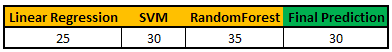
1. Simple Average
In this method, we take simple average (or mean) of the predicted probability on test data in case of classification model. If it is a regression model, calculate by taking mean of predicted values.
 |
| Ensemble : Simple Average |
2. Weighted Average
Unlike 'Simple Average' method, we do not assign equal weights. Instead we apply different weights to each of the algorithms. One of the way to calculate weights is to build logistic regression. See the steps below -
Step I : Multiple different algorithms are trained on training data. For example, Boosting Trees and Single Decision Tree were trained on a data set. These are the two classifiers.
Step II : Apply cross validation (k-fold) using training data. Let's say, you run 10 fold validation.
Step III : Calculate and save predicted probabilities from each of the 10 folds.
Step IV : Combine original dependent variable and two columns of the above predicted probabilities from boosting and decision tree.
Step V : Run Logistic Regression on data set prepared in step IV.
Step V : Capture two coefficients (ignoring intercept) derived from logistic regression.
Step VI : Calculate linear weights based on the coefficients.
Step VII : Predict on test data using trained models.
Step VIII : Calculate Ensemble Learning Prediction Probability Score by multiplying weights with predicted scores.
Step VI : Calculate linear weights based on the coefficients.
Weight I : abs(Coefficient I) / Sum (abs(Coefficient I) + abs(Coefficient II))In this step, we are calculating the overall importance of a variable. It is important to take absolute value of coefficients before calculating linear weights.
Weight II : abs(Coefficient I) / Sum (abs(Coefficient I) + abs(Coefficient II))
Step VII : Predict on test data using trained models.
Step VIII : Calculate Ensemble Learning Prediction Probability Score by multiplying weights with predicted scores.
Ensemble Learning = W1 * P1 + W2 * P2W1 : Weight of First Algorithm, W2 : Weight of Second Algorithm, P1 : Predicted Probability of First Algorithm, P2 : Predicted Probability of Second Algorithm
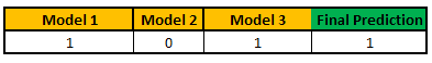
3. Majority Voting
Every model returns predicted probability on test data and the final prediction is the one that receives majority of the votes. If none of the predictions get more than half of the votes, we may say that the ensemble method could not make a stable prediction for this observation or case.
 |
| Ensemble : Majority Voting |
In this case we give higher weightage to the votes of one or more models. To find which models to assign higher weightage can be calculated using the logic we used for weighted average method.
5. Ensemble Stacking (aka Blending)
Stacking is an ensemble method where the models are combined using another data mining technique. Follow the steps below -
- Train multiple algorithms on training data. These models are known as bottom layer models
- Perform k-fold cross-validation using training data on each of these algorithms and save cross-validated predicted probabilities from each of these algorithms
- Train logistic regression or any machine learning algorithm on the cross- validated predicted probabilities in step 2 as independent variables and original target variable as dependent variable. In this case, trained model is a top layer model
- Make prediction from multiple trained models on test data
- Predict using the top layer model with the predictions of bottom layer models that has been made for testing data
6. Bagging
It is also called Bootstrap Aggregating. In this algorithm, it creates multiple models using the same algorithm but with random sub-samples of the dataset which are drawn from the original dataset randomly with random with replacement sampling technique (i..e. bootstrapping). This sampling method simply means some observations appear more than once while sampling. For example, Random Forest is a bagging algorithm.
7. Boosting
Boosting refers to boosting performance of weak models (decision tree). It involves the first algorithm is trained on the entire training data and the subsequent algorithms are built by fitting the residuals of the first algorithm, thus giving higher weight to those observations that were poorly predicted by the previous model. Adaboost, Gradient Boosting and Extreme Gradient Boosting are examples of this ensemble technique.
Ensembling : Weighted Average using Logistic Regression in R
In the code below, we are combining various models such as random forest, extremely randomized trees, Gradient Boosting Model, Support Vector Machine and Rotation Forest. Later we are applying linear weights which are calculated from logistic regression model.
#Combining Prediction probability of various models
finaldata = cbind(val_rf, val_ext_rf, val_gbm.tune, val_svm.tune, rotf_tune, target=val$Class2)
names(finaldata) = c("rf", "extr_rf", "gbm", "svm", "rotational", "target")
#Calculating Correlation Coefficient
descrCor <- cor(finaldata[-6])
descrCor
#Applying Logistic Regression
mylogistic <- glm(target ~ ., data = finaldata, family = "binomial")
summary(mylogistic)$coefficient
xx = data.frame(summary(mylogistic)$coefficient)
#Clean the coefficients
xx$variables = row.names(xx)
xx= xx[c("variables", "Estimate")][-1,]
#Calculate and applying Weights
xx$weight=abs(xx$weight)
xx$weight= xx$Estimate / sum(xx$Estimate)
finaldata$EnsemblePred = (xx$weight[1]*finaldata$rf) + (xx$weight[2]*finaldata$extr_rf) +
(xx$weight[3]*finaldata$gbm) + (xx$weight[4]*finaldata$svm + (xx$weight[5]*finaldata$rotational))
#Prediction is ROCR function
perf = prediction(finaldata$EnsemblePred, finaldata$target)
#performance in terms of true and false positive rates
# 1. Area under curve
auc = performance(perf, "auc")
auc
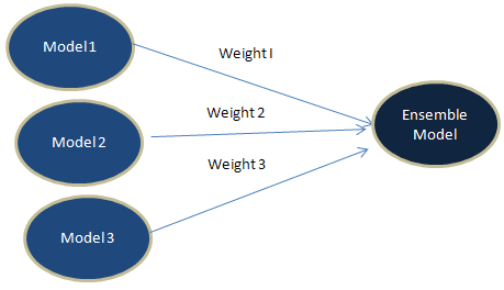
Ensembling : Weights with Neural Network
See the diagram below which visualizes how ensemble learning works -
 |
| Ensemble Learning |
We can use neural network to find optimal weights for stacking. It would calculate weights from input nodes to the output node. To accomplish this task, we can limit the number of hidden nodes to 1. It automatically adjusts the total sum of weights as 1. We can implement the same with R via deepnet package. See the code below for reference.
#Combine various modelsfinaldata = cbind(val_rf, val_trained_extrf, val_gbm.tune, val_svm.tune, rotf_tune)#Prepare independent and dependent variables in matrix formx <- as.matrix(finaldata)y <- as.numeric(ifelse(val$Class=="Abnormal",0,1))#Load Neural Network librarylibrary(deepnet)neuralnet <- dbn.dnn.train(x,y,hidden = c(1),activationfun = "sigm",learningrate = 0.2,momentum = 0.8)neuralnet_predict <- nn.predict(neuralnet,x)finaldata$NNPRed = neuralnet_predictfinaldata$y = y#prediction is ROCR functionperf = prediction(finaldata$NNPRed, finaldata$y)#performance in terms of true and false positive rates# Area under curveauc = performance(perf, "auc")auc
R : Building Model with Ensemble Stacking
In R, there is a package called caretEnsemble which makes ensemble stacking easy and automated. This package is an extension of most popular data science package caret. In the program below, we perform ensemble stacking manually (without use of caretEnsemble package).
# Loading Required Packages
library(caret)
library(caTools)
library(RCurl)
library(pROC)
# Reading data file
urlfile <-'https://raw.githubusercontent.com/hadley/fueleconomy/master/data-raw/vehicles.csv'
x <- getURL(urlfile, ssl.verifypeer = FALSE)
vehicles <- read.csv(textConnection(x))
# Cleaning up the data and only use the first 24 columns
vehicles <- vehicles[names(vehicles)[1:24]]
vehicles <- data.frame(lapply(vehicles, as.character), stringsAsFactors=FALSE)
vehicles <- data.frame(lapply(vehicles, as.numeric))
vehicles[is.na(vehicles)] <- 0
vehicles$cylinders <- ifelse(vehicles$cylinders == 6, 1,0)
# Making dependent variable factor and label values
vehicles$cylinders <- as.factor(vehicles$cylinders)
vehicles$cylinders <- factor(vehicles$cylinders,
levels = c(0,1),
labels = c("level1", "level2"))
# Split data into two sets - Training and Testing
set.seed(107)
inTrain <- createDataPartition(y = vehicles$cylinders, p = .7, list = FALSE)
training <- vehicles[ inTrain,]
testing <- vehicles[-inTrain,]
#Training control
ctrl <- trainControl(
method = "cv",
number = 3,
savePredictions = 'final',
classProbs = T
)
#Training decision tree
dt <-train(cylinders~., data=training, method="rpart",trControl=ctrl, tuneLength=2)
#Training logistic regression
logit <-train(cylinders~., data=training, method="glm",trControl=ctrl, tuneLength=2)
#Training knn model
knn <-train(cylinders~., data=training, method="knn",trControl=ctrl,tuneLength=2)
#Check Correlation Matrix of Accuracy
results <- resamples(list(dt, logit, knn))
modelCor(results)
#Predicting probabilities for testing data
testing$dt<- predict(dt,testing,type='prob')$level2
colAUC(testing$dt, testing$cylinders)
# 0.9358045
testing$logit<-predict(logit,testing,type='prob')$level2
colAUC(testing$logit, testing$cylinders)
# 0.5054634
testing$knn<-predict(knn,testing,type='prob')$level2
colAUC(testing$knn, testing$cylinders)
# 0.9871729
#Predicting the out of fold prediction probabilities for training data
#In this case, level2 is event
#rowindex : row numbers of the data used in k-fold
#Sorting by rowindex
training$OOF_dt<-dt$pred$level2[order(dt$pred$rowIndex)]
training$OOF_logit<-logit$pred$level2[order(logit$pred$rowIndex)]
training$OOF_knn<-knn$pred$level2[order(knn$pred$rowIndex)]
#GBM as top layer model
model_gbm<- train(training[,c('OOF_dt','OOF_logit','OOF_knn')],
training[,"cylinders"],method='gbm',trControl=ctrl,
tuneLength=1)
#Predict using GBM
testing$stacking<-predict(model_gbm, testing[,c('dt','logit','knn')], type = 'prob')$level2
colAUC(testing$stacking, testing$cylinders)
# 0.9903686
Important Point
We can also use logistic Regression for stacking. It uses simple linear classifier as compared to GBM. The sophistical models such as GBM are much more susceptible to overfitting while stacking.
Popularity of Ensemble Learning - Stacking
Endnotes
In the past, I have used this algorithm several times in real world data science projects. It helped to improve accuracy by 10 to 20%. But we need to be very cautious about it. Sometimes it leads to overfitting so we need to make sure we cross validated the result before implementing it in production. Please share your experience about it in the comment box below.
We can also use logistic Regression for stacking. It uses simple linear classifier as compared to GBM. The sophistical models such as GBM are much more susceptible to overfitting while stacking.
We should use Trees instead of Logistic Regression for an ensemble when we have :
- Lots of data
- Lots of models with similar accuracy scores
- Your models are uncorrelated (Accuracy/ROC in various samples of cross-validation). In case of regression, check correlation of residuals from multiple algorithms
The use of ensemble learning is very common in data science competitions such as Kaggle. Most of kagglers already know about this algorithm. They generally use it to improve their score. Also if you look at the solution of Kaggle competition winners, you would find the ensemble stacking being the top algorithm to combine multiple models. Ensemble stacking does not only improve accuracy of the model but also increase robustness of the model.
Endnotes
In the past, I have used this algorithm several times in real world data science projects. It helped to improve accuracy by 10 to 20%. But we need to be very cautious about it. Sometimes it leads to overfitting so we need to make sure we cross validated the result before implementing it in production. Please share your experience about it in the comment box below.

Deepanshu founded ListenData with a simple objective - Make analytics easy to understand and follow. He has over 10 years of experience in data science. During his tenure, he worked with global clients in various domains like Banking, Insurance, Private Equity, Telecom and HR.
Hi...
ReplyDeleteyou need to remove " n.minobsinnode = 10" from tuneList=list(....)
It was a great help in understanding the blending.
Thanks
Why should i remove - n.minobsinnode = 10? It is one of the tuning parameter of GBM.
DeleteIt works in the latest version of caret. Check out this link http://topepo.github.io/caret/training.html
Deleteok.
DeleteI was using the older version. By the way, very good post.
Cool. Glad you found it useful.
Deletethanks for sharing.. was very helpful..
ReplyDeletePlies send the data
ReplyDeleteHi,
ReplyDeleteI copied and pasted the code above and run it on my computer. I ran into this problem I couldn't figure out what went wrong. Attached is the code, and the last line is where the problem occurs.
# Loading Required Packages
library(caret)
library(caTools)
library(RCurl)
library(caretEnsemble)
library(pROC)
# Reading data file
urlfile <-'https://raw.githubusercontent.com/hadley/fueleconomy/master/data-raw/vehicles.csv'
x <- getURL(urlfile, ssl.verifypeer = FALSE)
vehicles <- read.csv(textConnection(x))
# Cleaning up the data and only use the first 24 columns
vehicles <- vehicles[names(vehicles)[1:24]]
vehicles <- data.frame(lapply(vehicles, as.character), stringsAsFactors=FALSE)
vehicles <- data.frame(lapply(vehicles, as.numeric))
vehicles[is.na(vehicles)] <- 0
vehicles$cylinders <- ifelse(vehicles$cylinders == 6, 1,0)
# Making dependent variable factor and label values
vehicles$cylinders <- as.factor(vehicles$cylinders)
vehicles$cylinders <- factor(vehicles$cylinders,
levels = c(0,1),
labels = c("level1", "level2"))
# Split data into two sets - Training and Testing
set.seed(107)
inTrain <- createDataPartition(y = vehicles$cylinders, p = .7, list = FALSE)
training <- vehicles[ inTrain,]
testing <- vehicles[-inTrain,]
# Setting Control
ctrl <- trainControl(
method='cv',
number= 3,
savePredictions=TRUE,
classProbs=TRUE,
index=createResample(training$cylinders, 10),
summaryFunction=twoClassSummary
)
# Train Models
model_list <- caretList(
cylinders~., data=training,
trControl = ctrl,
metric='ROC',
tuneList=list(
rf1=caretModelSpec(method='rpart', tuneLength = 10),
gbm1=caretModelSpec(method='gbm', distribution = "bernoulli",
bag.fraction = 0.5, tuneGrid=data.frame(n.trees = 50,
interaction.depth = 2,
shrinkage = 0.1,
n.minobsinnode = 10))
)
)
# Check AUC of Individual Models
model_list$rf1
model_list$gbm1
#Check the 2 model’s correlation
#Good candidate for an ensemble: their predictions are fairly uncorrelated,
#but their overall accuracy is similar
modelCor(resamples(model_list))
#################################################################
# Technique I : Stacking / Blending with GLM
#################################################################
glm_ensemble <- caretStack(
model_list,
method='glm',
metric='ROC',
trControl=trainControl(
method='cv',
number=3,
savePredictions=TRUE,
classProbs=TRUE,
summaryFunction=twoClassSummary
)
)
# Check Results
glm_ensemble
########################################################
# Validation on Testing Sample
########################################################
ensemble <- predict(glm_ensemble, newdata=testing, type='prob')$level2
When I ran the line above, I got the following message
" Error in eval(expr, envir, enclos) : object 'rf1' not found"
Please help. Thanks in advance.
Hi. First, I like to thank you for the great and easy to follow walkthrough. I have been able adapt this to several other algorithms and it works fine with expected results. However, I have challenges understanding what exactly this training$OOF_dt and this testing$dt are.
ReplyDeleteMy understanding is that, one is just a sorted form of the other and I know they form new columns in the training and testing sets.The confusing part is that you referred to "training$OOF_dt" as another prediction.
Thank you for responding.
Many thanks Deepanshu.
ReplyDeleteI have one question though. How can we use Grid (expand.grid) values for different algorithms?
Regards
Abhay
good post!, thanks
ReplyDelete