This tutorial explains how to create interactive chart with List Box.
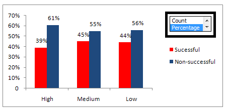 |
| Interactive Chart with List Box |
Steps
1. Prepare Data for Count and Percent
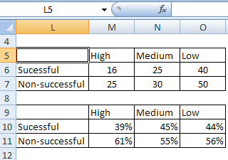 |
| Count and Percent Data |
2. Create
List Box
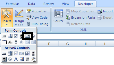 |
| Insert List Box |
3. Right click on List Box and go to
Control tab and give cell reference to
Input Range (Count and Percentage)
and Cell link.
Input Range - What do you want to display in List Box (Count Percentage)
Cell Link - the cell address where you do want to store value (1/2)
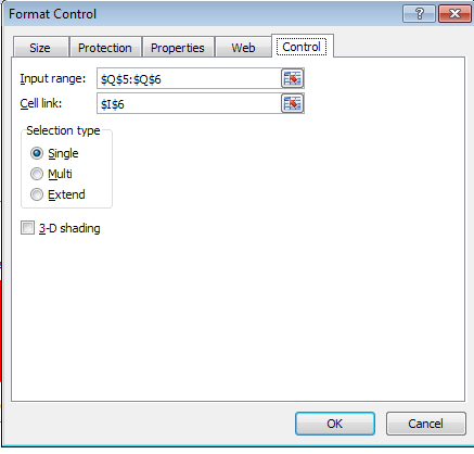 |
| List Box - Cell Reference |
4. Create Chart Range
=IF($I$6=1,M6,ROUND(M10,2))
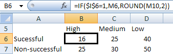 |
| Create Chart Range |
5. Add Custom Format to Chart Range
[>=1] #,##0;[>0] 0%;0
If a cell value is whole number, then add number format. Otherwise, use % format.
7. Create Chart
Select chart range and then press ALT N C and select column chart.
Download Excel Chart
About Author:
Deepanshu founded ListenData with a simple objective - Make analytics easy to understand and follow. He has over 10 years of experience in data science. During his tenure, he worked with global clients in various domains like Banking, Insurance, Private Equity, Telecom and HR.


Share Share Tweet