This tutorial would help you to learn Data Science with Python by examples. It is designed for beginners who want to get started with Data Science in Python. Python is an open source language and it is widely used as a high-level programming language for general-purpose programming. It has gained high popularity in data science world. In the PyPL Popularity of Programming language index, Python leads with a 29 percent share. In advanced analytics and predictive analytics market, it is ranked among top 3 programming languages for advanced analytics.
 |
| Data Science with Python Tutorial |
Introduction
Python is widely used and very popular for a variety of software engineering tasks such as website development, cloud-architecture, back-end etc. It is equally popular in data science world. In advanced analytics world, there has been several debates on R vs. Python. There are some areas such as number of libraries for statistical analysis, where R wins over Python but Python is catching up very fast.With popularity of big data and data science, Python has become first programming language of data scientists.There are several reasons to learn Python. Some of them are as follows -
- Python runs well in automating various steps of a predictive model.
- Python has awesome robust libraries for machine learning, natural language processing, deep learning, big data and artificial Intelligence.
- Python wins over R when it comes to deploying machine learning models in production.
- It can be easily integrated with big data frameworks such as Spark and Hadoop.
- Python has a great online community support.
- YouTube
- Dropbox
- Disqus
Python 2 vs. 3
Google yields thousands of articles on this topic. Some bloggers opposed and some in favor of 2.7. If you filter your search criteria and look for only recent articles, you would find Python 2 is no longer supported by the Python Software Foundation. Hence it does not make any sense to learn 2.7 if you start learning it today. Python 3 supports all the packages. Python 3 is cleaner and faster. It is a language for the future. It fixed major issues with versions of Python 2 series. Python 3 was first released in year 2008. It has been 12 years releasing robust versions of Python 3 series. You should go for latest version of Python 3.How to install Python?
There are two ways to download and install Python- Download Anaconda. It comes with Python software along with preinstalled popular libraries.
- Download Pythonfrom its official website. You have to manually install libraries.
Recommended : Go for first option and download anaconda. It saves a lot of time in learning and coding Python
- Jupyter (Ipython) Notebook
- Spyder
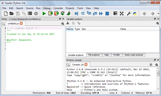 |
| Spyder - Python Coding Environment |
- Press F5 to run the entire script
- Press F9 to run selection or line
- Press Ctrl+ 1 to comment / uncomment
- Go to front of function and then press Ctrl + I to see documentation of the function
- Run %reset -f to clean workspace
- Ctrl + Left click on object to see source code
- Ctrl+Enter executes the current cell.
- Shift+Enter executes the current cell and advances the cursor to the next cell
| Arithmetic Operators | Operation | Example |
|---|---|---|
| + | Addition | 10 + 2 = 12 |
| – | Subtraction | 10 – 2 = 8 |
| * | Multiplication | 10 * 2 = 20 |
| / | Division | 10 / 2 = 5.0 |
| % | Modulus (Remainder) | 10 % 3 = 1 |
| ** | Power | 10 ** 2 = 100 |
| // | Floor | 17 // 3 = 5 |
| (x + (d-1)) // d | Ceiling | (17 +(3-1)) // 3 = 6 |
Basic programs in Python
#Basics
x = 10
y = 3
print("10 divided by 3 is", x/y)
print("remainder after 10 divided by 3 is", x%y)
Result :10 divided by 3 is 3.33
remainder after 10 divided by 3 is 1
x = 100
x > 80 and x <=95
x > 35 or x < 60
x > 80 and x <=95
Out[45]: False
x > 35 or x < 60
Out[46]: True
| Comparison & Logical Operators | Description | Example |
|---|---|---|
| > | Greater than | 5 > 3 returns True |
| < | Less than | 5 < 3 returns False |
| >= | Greater than or equal to | 5 >= 3 returns True |
| <= | Less than or equal to | 5 <= 3 return False |
| == | Equal to | 5 == 3 returns False |
| != | Not equal to | 5 != 3 returns True |
| and | Check both the conditions | x > 18 and x <=35 |
| or | If atleast one condition hold True | x > 35 or x < 60 |
| not | Opposite of Condition | not(x>7) |
Assignment Operators
It is used to assign a value to the declared variable. For e.g. x += 25 means x = x+25.
x = 100
y = 10
x += y
print(x)
print(x)
110
In this case, x+=y implies x=x+y which is x = 100+ 10.
Similarly, you can use x-=y, x*=y and x /=y
Python Data Structures
In every programming language, it is important to understand the data structures. Following are some data structures used in Python.- x = [1, 2, 3, 4, 5]
- y = [‘A’, ‘O’, ‘G’, ‘M’]
- z = [‘A’, 4, 5.1, ‘M’]
x = [1, 2, 3, 4, 5]
x[0]
x[1]
x[4]
x[-1]
x[-2]
x[0]
Out[68]: 1

x[1]
Out[69]: 2

x[4]
Out[70]: 5

x[-1]
Out[71]: 5

x[-2]
Out[72]: 4
x[0] picks first element from list. Negative sign tells Python to search list item from right to left. x[-1] selects the last element from list.
You can select multiple elements from a list using the following method
x[:3] returns[1, 2, 3]
- A tuple cannot be changed once constructed whereas list can be modified.
- A tuple is created by placing comma-separated values inside parentheses ( ). Whereas, list is created inside square brackets [ ]
K = (1,2,3)
State = ('Delhi','Maharashtra','Karnataka')
for i in State:
print(i)
Delhi
Maharashtra
Karnataka
Detailed Tutorial : Python Data Structures
- Function starts with def keyword followed by function name and ( )
- Function body starts with a colon (:) and is indented
- The keyword return ends a function andgive value of previous expression.
def sum_fun(a, b):
result = a + b
return result
z = sum_fun(10, 15)Result : z = 25
Suppose you want python to assume 0 as default value if no value is specified for parameter b.
def sum_fun(a, b=0):
result = a + b
return result
z = sum_fun(10)
In the above function, b is set to be 0 if no value is provided for parameter b. It does not mean no other value than 0 can be set here. It can also be used asz = sum_fun(10, 15)
Note : The if and else statements ends with a colon :
k = 27
if k%5 == 0:
 print('Multiple of 5')
else:
 print('Not a Multiple of 5')
Result :Not a Multiple of 5List of popular packages (comparison with R)
Some of the leading packages in Python along with equivalent libraries in R are as follows-- pandas. For data manipulation and data wrangling. A collections of functions to understand and explore data. It is counterpart of dplyr and reshape2 packages in R.
- NumPy. For numerical computing. It's a package for efficient array computations. It allows us to do some operations on an entire column or table in one line. It is roughly approximate to Rcpp package in R which eliminates the limitation of slow speed in R. Numpy Tutorial
- Scipy.For mathematical and scientific functions such asintegration, interpolation, signal processing, linear algebra, statistics, etc. It is built on Numpy.
- Scikit-learn. A collection of machine learning algorithms. It is built on Numpy and Scipy. It can perform all the techniques that can be done in R usingglm, knn, randomForest, rpart, e1071 packages.
- Matplotlib.For data visualization. It's a leading package for graphics in Python. It is equivalent to ggplot2 package in R.
- Statsmodels.For statistical and predictive modeling. It includes various functions to explore data and generate descriptive and predictive analytics. It allows users to run descriptive statistics, methods to impute missing values, statistical tests and take table output to HTML format.
- pandasql. It allows SQL users to write SQL queries in Python. It is very helpful for people who loves writing SQL queries to manipulate data. It is equivalent to sqldf package in R.
| Task | Python Package | R Package |
|---|---|---|
| IDE | Rodeo / Spyder | Rstudio |
| Data Manipulation | pandas | dplyr and reshape2 |
| Machine Learning | Scikit-learn | glm, knn, randomForest, rpart, e1071 |
| Data Visualization | ggplot + seaborn + bokeh | ggplot2 |
| Character Functions | Built-In Functions | stringr |
| Reproducibility | Jupyter | Knitr |
| SQL Queries | pandasql | sqldf |
| Working with Dates | datetime | lubridate |
| Web Scraping | beautifulsoup | rvest |
Popular python commands
The commands below would help you to install and update new and existing packages. Let's say, you want to install / uninstall pandas package.!pip install pandas
Uninstall Package
!pip uninstall pandas
Show Information about Installed Package
!pip show pandas
List of Installed Packages
!pip list
Upgrade a package
!pip install --upgrade pandas --user
1. import pandas as pd It imports the package pandas under the alias pd. A function DataFrame in package pandas is then submitted with pd.DataFrame.
2. import pandas
It imports the package without using alias but here the function DataFrame is submitted with full package name pandas.DataFrame
3. from pandas import *
It imports the whole package and the function DataFrame is executed simply by typing DataFrame. It sometimes creates confusion when same function name exists in more than one package.
import pandas as pd
import numpy as  np
s1 = pd.Series(np.random.randn(5))
s1
0   -2.412015
1   -0.451752
2    1.174207
3    0.766348
4   -0.361815
dtype: float64
s1[0]
-2.412015s1[1]
-0.451752s1[:3]
0   -2.412015
1   -0.451752
2    1.174207
It is equivalent to data.frame in R. It is a 2-dimensional data structure that can store data of different data types such as characters, integers, floating point values, factors. Those who are well-conversant with MS Excel, they can think of data frame as Excel Spreadsheet.
| Data Type | Pandas | Standard Python |
|---|---|---|
| For character variable | object | string |
| For categorical variable | category | - |
| For Numeric variable without decimals | int64 | int |
| Numeric characters with decimals | float64 | float |
| For date time variables | datetime64 | - |
Important Pandas Functions (vs. R functions)
The table below shows comparison of pandas functions with R functions for various data wrangling and manipulation tasks. It would help you to memorize pandas functions. It's a very handy information for programmers who are new to Python. It includes solutions for most of the frequently used data exploration tasks.| Functions | R | Python (pandas package) |
|---|---|---|
| Installing a package | install.packages('name') | !pip install name |
| Loading a package | library(name) | import name as other_name |
| Checking working directory | getwd() | import os os.getcwd() |
| Setting working directory | setwd() | os.chdir() |
| List files in a directory | dir() | os.listdir() |
| Remove an object | rm('name') | del object |
| Select Variables | select(df, x1, x2) | df[['x1', 'x2']] |
| Drop Variables | select(df, -(x1:x2)) | df.drop(['x1', 'x2'], axis = 1) |
| Filter Data | filter(df, x1 >= 100) | df.query('x1 >= 100') |
| Structure of a DataFrame | str(df) | df.info() |
| Summarize dataframe | summary(df) | df.describe() |
| Get row names of dataframe "df" | rownames(df) | df.index |
| Get column names | colnames(df) | df.columns |
| View Top N rows | head(df,N) | df.head(N) |
| View Bottom N rows | tail(df,N) | df.tail(N) |
| Get dimension of data frame | dim(df) | df.shape |
| Get number of rows | nrow(df) | df.shape[0] |
| Get number of columns | ncol(df) | df.shape[1] |
| Length of data frame | length(df) | len(df) |
| Get random 3 rows from dataframe | sample_n(df, 3) | df.sample(n=3) |
| Get random 10% rows | sample_frac(df, 0.1) | df.sample(frac=0.1) |
| Check Missing Values | is.na(df$x) | pd.isnull(df.x) |
| Sorting | arrange(df, x1, x2) | df.sort_values(['x1', 'x2']) |
| Rename Variables | rename(df, newvar = x1) | df.rename(columns={'x1': 'newvar'}) |
Examples - Data analysis with Pandas
import numpy as np
import pandas as pd
mydata = {'productcode': ['AA', 'AA', 'AA', 'BB', 'BB', 'BB'],
sales': [1010, 1025.2, 1404.2, 1251.7, 1160, 1604.8],
cost' : [1020, 1625.2, 1204, 1003.7, 1020, 1124]}
df = pd.DataFrame(mydata)
In this dataframe, we have three variables - productcode, sales, cost.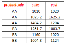 |
| Sample DataFrame |
mydata= pd.read_csv("C:\\Users\\Deepanshu\\Documents\\file1.csv")Make sure you use double backslash when specifying path of CSV file. Alternatively, you can use forward slash to mention file path inside read_csv() function.
df.shapeResult :(6, 3). It means 6 rows and 3 columns.
df.head(3)
     cost productcode   sales
0  1020.0          AA  1010.0
1  1625.2          AA  1025.2
2  1204.0          AA  1404.2
To keep a single variable, you can write in any of the following three methods -
df.productcodeTo select variable by column position, you can use df.iloc function. In the example below, we are selecting second column. Column Index starts from 0. Hence, 1 refers to second column.
df["productcode"]
df.loc[: , "productcode"]
df.iloc[: , 1]We can keep multiple variables by specifying desired variables inside [ ]. Also, we can make use of df.loc() function.
df[["productcode", "cost"]]
df.loc[ : , ["productcode", "cost"]]
Drop Variable
We can remove variables by using df.drop() function. See the example below -
df2 = df.drop(['sales'], axis = 1)
To summarize or explore data, you can submit the command below.
df.describe()
              cost       sales
count     6.000000     6.00000
mean   1166.150000  1242.65000
std     237.926793   230.46669
min    1003.700000  1010.00000
25%    1020.000000  1058.90000
50%    1072.000000  1205.85000
75%    1184.000000  1366.07500
max    1625.200000  1604.80000
To summarise all the character variables, you can use the following script.
df.describe(include=['O'])Similarly, you can use df.describe(include=['float64']) to view summary of all the numeric variables with decimals.
To select only a particular variable, you can write the following code -
df.productcode.describe()
OR
df["productcode"].describe()
count      6
unique     2
top       BB
freq       3
Name: productcode, dtype: object
df.sales.mean()
df.sales.median()
df.sales.count()
df.sales.min()
df.sales.max()
df1 = df[(df.productcode == "AA") & (df.sales >= 1250)]It can also be written like :
df1 = df.query('(productcode == "AA") & (sales >= 1250)')In the second query, we do not need to specify DataFrame along with variable name.
df.sort_values(['sales'])
df.groupby(df.productcode).mean()
                    cost        sales
productcode
AA           1283.066667  1146.466667
BB           1049.233333  1338.833333
Instead of summarising for multiple variable, you can run it for a single variable i.e. sales. Submit the following script.
df["sales"].groupby(df.productcode).mean()
df0 = pd.DataFrame({'id': [1, 1, 2, 3, 1, 2, 2]})Let's define as a categorical variable.
We can use astype() function to make id as a categorical variable.
df0.id = df0["id"].astype('category')Summarize this classification variable to check descriptive statistics.
df0.describe()
       id
count    7
unique   3
top      2
freq     3
df['productcode'].value_counts()
BB    3
AA    3
df['sales'].hist()
 |
| Histogram |
df.boxplot(column='sales')
 |
| BoxPlot |
#Import required libraries
import pandas as pd
import statsmodels.api as sm
import numpy as np
# Read data from web
df = pd.read_csv("https://stats.idre.ucla.edu/stat/data/binary.csv")
Variables Type Description
gre Continuous Graduate Record Exam score
gpa Continuous Grade Point Average
rank Categorical Prestige of the undergraduate institution
admit Binary Admission in graduate school
The binary variable admit is a target variable.
- How many rows and columns in the data file?
- What are the distribution of variables?
- Check if any outlier(s)
- If outlier(s), treat them
- Check if any missing value(s)
- Impute Missing values (if any)
# See no. of rows and columnsResult : 400 rows and 4 columns
df.shape
In the code below, we rename the variable rank to 'position' as rank is already a function in python.
# rename rank columnSummarize and plot all the columns.
df = df.rename(columns={'rank': 'position'})
# Summarize
df.describe()
# plot all of the columns
df.hist()
# Summarize
df.position.value_counts(ascending=True)
1     61
4     67
3    121
2    151
pd.crosstab(df['admit'], df['position'])
position   1   2   3   4
admit
0         28  97  93  55
1         33  54  28  12
for i in list(df.columns) :In this case, there are no missing values in the dataset.
k = sum(pd.isnull(df[i]))
print(i, k)
Data Science with Python
In this section we covered how we can build predictive model using common statistical modeling techniques. It also includes data processing steps prior to model development and validation.Logistic Regression
Logistic Regression is a special type of regression where target variable is categorical in nature and independent variables be discrete or continuous. In this post, we will demonstrate only binary logistic regression which takes only binary values in target variable. Unlike linear regression, logistic regression model returns probability of target variable.It assumes binomial distribution of dependent variable. In other words, it belongs to binomial family.
In python, we can write R-style model formula y ~ x1+ x2+ x3 using patsy and statsmodels libraries. In the formula, we need to define variable 'position' as a categorical variable by mentioning it inside capital C(). You can also define reference category using reference= option.
#Reference CategoryIt returns two datasets - X and y. The dataset 'y' contains variable admit which is a target variable. The other dataset 'X' contains Intercept (constant value), dummy variables for Treatment, gre and gpa. Since 4 is set as a reference category, it will be 0 against all the three dummy variables. See sample below -
from patsy import dmatrices, Treatment
y, X = dmatrices('admit ~ gre + gpa + C(position, Treatment(reference=4))', df, return_type = 'dataframe')
P  P_1 P_2 P_3
3  0 0 1
3  0 0 1
1  1 0 0
4  0 0 0
4  0 0 0
2  0 1 0
from sklearn.model_selection import train_test_split
X_train, X_test, y_train, y_test = train_test_split(X, y, test_size=0.2, random_state=0)
#Fit Logit model logit = sm.Logit(y_train, X_train) result = logit.fit() #Summary of Logistic regression model result.summary() result.params
                          Logit Regression Results
==============================================================================
Dep. Variable:                  admit   No. Observations:                  320
Model:                          Logit   Df Residuals:                      315
Method:                           MLE   Df Model:                            4
Date:                Sat, 20 May 2017   Pseudo R-squ.:                 0.03399
Time:                        19:57:24   Log-Likelihood:                -193.49
converged:                       True   LL-Null:                       -200.30
                                        LLR p-value:                  0.008627
=======================================================================================
                      coef    std err          z       P|z|      [95.0% Conf. Int.]
---------------------------------------------------------------------------------------
C(position)[T.1]     1.4933      0.440      3.392      0.001         0.630     2.356
C(position)[T.2]     0.6771      0.373      1.813      0.070        -0.055     1.409
C(position)[T.3]     0.1071      0.410      0.261      0.794        -0.696     0.910
gre                  0.0005      0.001      0.442      0.659        -0.002     0.003
gpa                  0.4613      0.214     -2.152      0.031        -0.881    -0.041
======================================================================================
#Confusion Matrix
result.pred_table()
#Odd Ratio
np.exp(result.params)
#prediction on test data
y_pred = result.predict(X_test)
# AUC on test dataResult : AUC =0.6763
false_positive_rate, true_positive_rate, thresholds = roc_curve(y_test, y_pred)
auc(false_positive_rate, true_positive_rate)
accuracy_score([ 1 if p > 0.5 else 0 for p in y_pred ], y_test)
Decision Tree
Decision trees can have a target variable continuous or categorical. When it is continuous, it is called regression tree. And when it is categorical, it is called classification tree. It selects a variable at each step that best splits the set of values. There are several algorithms to find best split. Some of them are Gini, Entropy, C4.5, Chi-Square. There are several advantages of decision tree. It is simple to use and easy to understand. It requires a very few data preparation steps. It can handle mixed data - both categorical and continuous variables. In terms of speed, it is a very fast algorithm.#Drop Intercept from predictors for tree algorithms X_train = X_train.drop(['Intercept'], axis = 1) X_test = X_test.drop(['Intercept'], axis = 1) #Decision Tree from sklearn.tree import DecisionTreeClassifier model_tree = DecisionTreeClassifier(max_depth=7) #Fit the model: model_tree.fit(X_train,y_train) #Make predictions on test set predictions_tree = model_tree.predict_proba(X_test) #AUC false_positive_rate, true_positive_rate, thresholds = roc_curve(y_test, predictions_tree[:,1]) auc(false_positive_rate, true_positive_rate)Result : AUC = 0.664
Feature engineering plays an important role in building predictive models. In the above case, we have not performed variable selection. We can also select best parameters by using grid search fine tuning technique.
Random Forest
Decision Tree has limitation of overfitting which implies it does not generalize pattern. It is very sensitive to a small change in training data. To overcome this problem, random forest comes into picture. It grows a large number of trees on randomised data. It selects random number of variables to grow each tree. It is more robust algorithm than decision tree. It is one of the most popular machine learning algorithm. It is commonly used in data science competitions. It is always ranked in top 5 algorithms. It has become a part of every data science toolkit.#Random Forest from sklearn.ensemble import RandomForestClassifier model_rf = RandomForestClassifier(n_estimators=100, max_depth=7) #Fit the model: target = y_train['admit'] model_rf.fit(X_train,target) #Make predictions on test set predictions_rf = model_rf.predict_proba(X_test) #AUC false_positive_rate, true_positive_rate, thresholds = roc_curve(y_test, predictions_rf[:,1]) auc(false_positive_rate, true_positive_rate) #Variable Importance importances = pd.Series(model_rf.feature_importances_, index=X_train.columns).sort_values(ascending=False) print(importances) importances.plot.bar()
Result : AUC = 0.6974
Grid Search - Hyper Parameter Tuning
The sklearn library makes hyper-parameters tuning very easy. It is a strategy to select the best parameters for an algorithm. In scikit-learn they are passed as arguments to the constructor of the estimator classes. For example, max_features in randomforest. alpha for lasso.from sklearn.model_selection import GridSearchCV
rf = RandomForestClassifier()
target = y_train['admit']
param_grid = {
'n_estimators': [100, 200, 300],
'max_features': ['sqrt', 3, 4]
}
CV_rfc = GridSearchCV(estimator=rf , param_grid=param_grid, cv= 5, scoring='roc_auc')
CV_rfc.fit(X_train,target)
#Parameters with Scores
CV_rfc.grid_scores_
#Best Parameters
CV_rfc.best_params_
CV_rfc.best_estimator_
#Make predictions on test set
predictions_rf = CV_rfc.predict_proba(X_test)
#AUC
false_positive_rate, true_positive_rate, thresholds = roc_curve(y_test, predictions_rf[:,1])
auc(false_positive_rate, true_positive_rate)
Cross Validation
# Cross Validation
from sklearn.linear_model import LogisticRegression
from sklearn.model_selection import cross_val_predict,cross_val_score
target = y['admit']
prediction_logit = cross_val_predict(LogisticRegression(), X, target, cv=10, method='predict_proba')
#AUC
cross_val_score(LogisticRegression(fit_intercept = False), X, target, cv=10, scoring='roc_auc')
Preprocessing Steps
1. The machine learning package sklearn requires all categorical variables in numeric form. Hence, we need to convert all character/categorical variables to be numeric. This can be accomplished using the following script. In sklearn, there is already a function for this step.from sklearn.preprocessing import LabelEncoder
def ConverttoNumeric(df):
cols = list(df.select_dtypes(include=['category','object']))
le = LabelEncoder()
for i in cols:
try:
df[i] = le.fit_transform(df[i])
except:
print('Error in Variable :'+i)
return df
ConverttoNumeric(df)
 |
| Encoding |
productcode_dummy = pd.get_dummies(df["productcode"])
df2 = pd.concat([df, productcode_dummy], axis=1)
The output looks like below -
   AA  BB
0   1   0
1   1   0
2   1   0
3   0   1
4   0   1
5   0   1
To avoid multi-collinearity, you can set one of the category as reference category and leave it while creating dummy variables. In the script below, we are leaving first category.
productcode_dummy = pd.get_dummies(df["productcode"], prefix='pcode', drop_first=True)
df2 = pd.concat([df, productcode_dummy], axis=1)
# fill missing values with 0
df['var1'] = df['var1'].fillna(0)
# fill missing values with mean
df['var1'] = df['var1'].fillna(df['var1'].mean())
from sklearn.preprocessing import Imputer
# Set an imputer object
mean_imputer = Imputer(missing_values='NaN', strategy='mean', axis=0)
# Train the imputor
mean_imputer = mean_imputer.fit(df)
# Apply imputation
df_new = mean_imputer.transform(df.values)
- Cap extreme values at 95th / 99th percentile depending on distribution
- Apply log transformation of variables. See below the implementation of log transformation in Python.
import numpy as np
df['var1'] = np.log(df['var1'])
#load dataset
dataset = load_boston()
predictors = dataset.data
target = dataset.target
df = pd.DataFrame(predictors, columns = dataset.feature_names)

#Apply Standardization
from sklearn.preprocessing import StandardScaler
k = StandardScaler()
df2 = k.fit_transform(df)
Next Step - Practice, practice and practice. Download free public data sets from Kaggle / UCLA websites and try to play around with data and generate insights from it with pandas package and build statistical models using sklearn package. I hope you would find this tutorial helpful. I tried to cover all the important topics which beginner must know about Python. Once completion of this tutorial, you can flaunt you know how to program it in Python and you can implement machine learning algorithms using sklearn package.

Deepanshu founded ListenData with a simple objective - Make analytics easy to understand and follow. He has over 10 years of experience in data science. During his tenure, he worked with global clients in various domains like Banking, Insurance, Private Equity, Telecom and HR.
Hi, excelent tutorial!!! I'm mostly a user of R but want to learn python. The thing is i work a lot with spatial data: spatial relationships (spdep), interpolation (kriging with gstat or multilevel B-Splines with MBA) etc.; and then machine learning methods with the data that comes from spatial features.
ReplyDeleteI understand that the ML cappabilities are already in Pythoon but i'm worried about the spatial workflow, can you give me some insights on this?
Thanks,
Great blog!
Thanks for developing this. For first time after few attempts, I can start working with Python!
ReplyDeleteGlad you found it helpful. Cheers!
DeleteHi Deepanshu. Can i have your contact number please. I want to talk regarding the courses.
DeleteThanks. Some things come late in the tutorial (like the np loading) but it is a good overview.
ReplyDeleteExcelent! I appreciate the comparison between R and Python commands! Very useful!
ReplyDeleteVery well written article!
ReplyDeleteHi.
ReplyDeleteI am using Pythin 3.6.
y, X = dmatrices("admit ~ gre + gpa + C(position, Treatment(reference=4))", df, return_type = 'dataframe')
This code generate this error
C, including its class ClassRegistry, has been deprecated since SymPy
1.0. It will be last supported in SymPy version 1.0. Use direct
imports from the defining module instead. See
https://github.com/sympy/sympy/issues/9371 for more info.
.
.
.
TypeError: 'bool' object is not callable
How can I handle this ?
Thank you
Very useful tutorial, lucidly presented
ReplyDelete⏳⛳🏳🚩🏁⛖🔛✖➕➖➗⁉⚌⚲
ReplyDeleteThanks for an amazing introduction to Python.
ReplyDeleteThank you for this interesting tutorial.
ReplyDeleteNicely written.. Thanks
ReplyDeleteExcellent resources to get hands on quick with Python
ReplyDeleteVery useful tutorial, lucidly presented
ReplyDeletehi while i am running
ReplyDeleteimport pandas as pd
s1 = pd.Series(np.random.randn(5))
s1
Its gives out an error as "np is not defined".
can you please rectify?
you also need to submit "import numpy as np" before pd.series()
DeleteHey there, you have to import numpy as well
Deletene pulse ultra for beginners
ReplyDeletesir..my doubt is that "Do we need to worry about removal of variables based on multicollinearity or the sklearn will take care of it automatically"
ReplyDeleteWe need to handle multicollinearity issue. Sklearn package would not take care of it automatically.
Deletegreat one!
ReplyDeleteI enjoyed reading through your post, The way of explanation about the comparison between R and Python is nice.
ReplyDeleteKeep working ,great job!
Excellent tutorial.....
ReplyDeleteBro Listendata is my fav blog for datascience. I have already learnt R using your tutorials, now I am learning Python. I am extremely thankful to you for such amazing content.
ReplyDeleteGod bless you and Lots of love!!!!!
dont judje mi spelling
ReplyDeleteModification as per my observation in Logistic regression
ReplyDelete(1) The other dataset 'X' contains Intercept (constant value), dummy variables for Treatment, gre and gpa. It may may right to modify this statement like
The other dataset 'X' contains Intercept (constant value), gre, gpa and dummy variables for Treatment
(2) In logistic regression these two module need to import
from sklearn.metrics import roc_curve
from sklearn.metrics import auc
Truly impressive. I cannot thank you enough.
ReplyDeleteGreat content useful for all the candidates of Data Science training who want to kick start these career in Data Science training field.
ReplyDeleteExcellent post,Keep sharing such type of wonderful post..
ReplyDeletecame across this in my coding journey, good read
ReplyDeleteThanks for sharing such a valuable blog.
ReplyDelete