In this article we will cover how to calculate AUC (Area Under Curve) in R.
What is Area Under Curve?
The Area Under Curve (AUC) is a metric used to evaluate the performance of a binary classification model. It measures the ability of a model to distinguish between events and non-events.
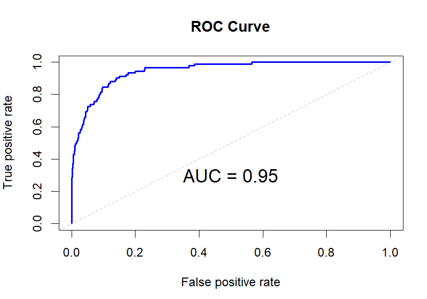
The AUC (ROC) curve is created by plotting the true positive rate (sensitivity) against the false positive rate (1-specificity) at various classification thresholds. The true positive rate is the proportion of events correctly classified as events, and the false positive rate is the proportion of non-events incorrectly classified as events.
The AUC ranges from 0 to 1, where:
- AUC = 0.5: The classifier performs no better than random chance.
- AUC > 0.5 and ≤ 1: The classifier performs better than random chance. A higher AUC value indicates better performance, with 1 representing a perfect classifier.
We need to have two R packages named ISLR and ROCR installed as prerequisites. If they are not already installed, you can install them using the command.
install.packages("ISLR")
install.packages("ROCR")
The performance() function from ROCR package is used to calculate the Area Under the Curve (AUC) as a performance metric for the model. The following R code builds logistic regression model for binary classification on the "Default" dataset from the "ISLR" package and then calculates AUC.
library(ISLR)
library(ROCR)

# Load a binary classification dataset from ISLR package
mydata <- ISLR::Default

# Set seed
set.seed(1234)

# 70% of dataset goes to training data and remaining 30% to test data
train_idx  <- sample(c(TRUE, FALSE), nrow(mydata), replace=TRUE, prob=c(0.7,0.3))
train <- mydata[train_idx, ]
test <- mydata[!train_idx, ]

# Build logistic regression model
model <- glm(default~., family="binomial", data=train)

# Calculate predicted probability of default of test data
predicted <- predict(model, test, type="response")

# Storing Model Performance Scores
pred  <- prediction(predicted, test$default)

# Calculating Area under Curve
perf <- performance(pred,"auc")
auc <- as.numeric(perf@y.values)
auc
Result: 0.9466106
- The "Default" dataset is loaded from the "ISLR" package.
- A seed is set using
set.seed(1234)to ensure reproducibility. It means same output will be generated in every run. - The dataset is split into a training set (70%) and a test set (30%) using random sampling.
- A logistic regression model is built using the
glmfunction, where "default" is the binary dependent variable, and the rest of the variables are used as independent variables. - The
predictfunction is used to calculate the predicted probabilities of default for the test data based on the logistic regression model. - The "ROCR" package is used to create a prediction object (pred) based on the predicted probabilities and the true default values from the test set.
- The performance of the model is evaluated by calculating the Area Under the Curve (AUC) using the
performancefunction from "ROCR."
Let's see how we can plot the ROC curve in R. In the following code, we first calculate the ROC curve using the performance function with "tpr" (True Positive Rate or Sensitivity) and "fpr" (False Positive Rate) as arguments. Then, we use the plot function to plot the ROC curve. The abline function is used to draw the diagonal line from (0,0) to (1,1), representing the ROC curve of a random classifier.
# Plot ROC curve
roc_curve <- performance(pred, "tpr", "fpr")
plot(roc_curve, col = "blue", main = "ROC Curve", lwd = 2)
abline(0, 1, col = "gray", lty = 2, lwd = 1)
text(0.5, 0.3, paste("AUC =", round(auc, 2)), adj = c(0.5, 0.5), col = "black", cex = 1.5)


Share Share Tweet