This article shows you two simple ways to increment the formula row when you copy it across different columns in Excel. It helps you understand how to manage your formulas better and make accurate calculations in your spreadsheets.
Suppose you are asked to calculate cumulative sale. And the figure should be displayed in columns. Hence the formula should increment by row when you copy it horizontally.

You can combine the OFFSET and COLUMN functions in Excel to create a dynamic reference that adjusts based on the column position.
=SUM(OFFSET($A$1,0,0,COLUMN(B1)))
Let's understand OFFSET and COLUMN functions
The Excel syntax for the OFFSET function is:=OFFSET(reference,rows,columns,[height],[width])It returns a reference to a range, from a given starting point with given height and width in cells.
- Reference - It is the starting point in range.
- Rows - These are the number of rows you want Excel to move from the starting point.
- Columns - These are the number of columns you want Excel to move from the starting point.
- Height [Optional] - It is the size of range with number of rows tall you want to return.
- Width [Optional] - It is the size of range with number of columns wide you want to return.
OFFSET(A1,0,0,2)From A1 returns 2 rows tall range. That means A1:A2
OFFSET(A1,0,0,1,2)From A1 returns 2 columns wide range. That means A1:B1
OFFSET(A1,0,0,2,2)From A1 returns 2 rows tall and 2 columns wide range. That means A1:B2.
OFFSET(A1,1,0)It means move down 1 row i.e. A2. Since height and width components are optional in OFFSET formula, you can skip their references.
OFFSET(A1,0,2)It means move right 2 columns i.e. C1.
SUM(OFFSET(A1,1,2,2,1))It means move down 1 row, 2 columns and then select 2 X 1 range. That means C2:C3.
=COLUMN(reference)
It returns the column number of a reference.
Examples :
1. COLUMN(A1) returns 1.
2. COLUMN(B1) returns 2.
Evaluate Formula :
Let's translate the following formula into English :
=SUM(OFFSET($A$1,0,0,COLUMN(B1)))Since COLUMN(B1) returns 2, the above formula means = SUM (A1 through 2 rows wide). That is equivalent to =SUM(A1:A2) When you copy the above formula across columns, the column formula increments by one.
=SUM(OFFSET($A$1,0,0,COLUMN(C1)))That is equivalent to = SUM(A1:A3)
You can combine the INDIRECT and ADDRESS functions in Excel to create a dynamic reference to a cell based on its row and column numbers.
=SUM(INDIRECT(ADDRESS(1,1)&":"&ADDRESS(COLUMN(B1),1)))Let's understand INDIRECT and ADDRESS functions
The Excel syntax for the INDIRECT function is: =INDIRECT(reference)
It allows you to change the reference to a cell within a formula without changing the formula itself.
Examples :
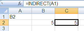
1. If cell A1 has the value "B2", then =INDIRECT(A1) will return the value in B2.

2. =SUM(INDIRECT("A1:A2")) --- INDIRECT function changes a text string to a reference. Let's evaluate this formula. = SUM(A1:A2)
The Excel syntax for the ADDRESS function is:
=ADDRESS (row_num, col_num, ref_type, ref_style, sheet_name)It returns the address for a cell when provided a row and a column number.
1. row_num - It is the row number to use in the cell reference. For example, 3 for row 3
2. col_num - It is the column number to use in the cell reference. For example, 3 for column C
3. ref_type [Optional]- It is the type of address you want to return.
- 1 or omitted for absolute (For example, $A$1)
- 2 for absolute row, relative column (For example, A$1)
- 3 for relative row, absolute column (For example, $A1)
- 4 for relative (For example, A1)
5. sheet_name [Optional] - It is the name of the worksheet to be used as the external reference. For example, "Sheet2"
Examples :
1. ADDRESS(2,1) means $A$2 2. ADDRESS(1,3,2) means C$1
= SUM(INDIRECT(ADDRESS(1,1)&":"&ADDRESS(COLUMN(B1),1)))
= SUM(INDIRECT("$A$1:$A$2"))
= SUM($A$1:$A$2)
Download the workbook


Oh Great you save my lots of real time
ReplyDelete