This article explains how to identify and interpret a right skewed histogram with examples.
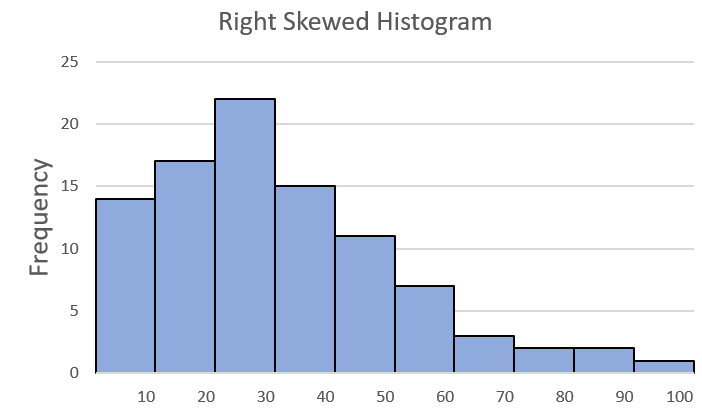
A right skewed histogram is a histogram where the tail on the right side is longer than usual, and the highest point (peak) of the graph is towards the left. In this situation, the smaller values appear more often in the data, while the larger values are not as common. It is also known as positively skewed histogram.
Properties of Right Skewed Histogram
Here are main properties of a right skewed histogram:
- Mean, Median and Mode: In a right-skewed distribution, the mode (most frequently occurring value) will be less than the median (middle value), and the median will be less than the mean.
Mean ≥ Median ≥ Mode

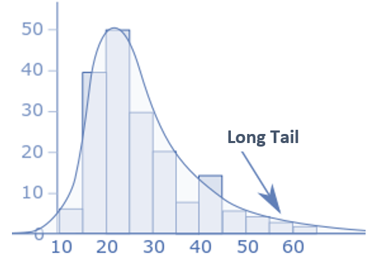
- Long Right Tail: The right-skewed histogram will have a long tail on the right-hand side, indicating that there are a few data points that are much larger than the majority of the data.
Reasons for Right Skewed Histogram
Let's understand what leads to a right skewed histogram.
- Few High Values: There will be a few data points with high values that contribute to the extended right tail. These high values can significantly impact the mean, causing it to be greater than the median. For example, imagine a group of people's incomes. Most of them earn average amounts, but a few earn a lot more. These high earners pull the overall average up, making it larger than what most people actually earn, which is shown by the middle value.
- Majority of Data on the Left: Most of the data points are positioned towards the left side of the histogram, indicating that the lower values are more common in the dataset.
Examples of Right Skewed Histogram
Here is a list of real-world examples that display a right skewed histogram:
1. Income Distribution: In many countries, a majority of people earn regular to decent incomes, while a smaller number of individuals earn extremely high incomes, causing the distribution to be right-skewed.
Let's take income of 10 individuals as shown in the table below and compare mean and median based on the data.
Mean: $62,000
Median: $52,500
| Income (in $) |
|---|
| 30,000 |
| 35,000 |
| 40,000 |
| 45,000 |
| 50,000 |
| 55,000 |
| 75,000 |
| 80,000 |
| 90,000 |
| 120,000 |
2. Age at Retirement: The majority of individuals tend to retire at around a certain age, but there are a few who retire much later, causing a right-skewed distribution of retirement ages.
Let's find out the mean, median and mode retirement age based on the following data.
Mean: 59.5
Median: 55
Mode: 55
| Retirement Age |
|---|
| 50 |
| 50 |
| 55 |
| 55 |
| 55 |
| 55 |
| 60 |
| 65 |
| 70 |
| 80 |
3. Test Scores: In education, test scores often follow a right-skewed distribution. Most students score around the average, but a few exceptional students achieve very high scores.

Deepanshu founded ListenData with a simple objective - Make analytics easy to understand and follow. He has over 10 years of experience in data science. During his tenure, he worked with global clients in various domains like Banking, Insurance, Private Equity, Telecom and HR.
Share Share Tweet