In this tutorial, you will learn how to apply OFFSET function in MS Excel.
The Excel syntax for the OFFSET function is:
=OFFSET(reference, rows, columns, [height], [width])
It returns a reference to a range, from a given starting point with given height and width in cells.
1. Reference - Starting point in range.
2. Rows - Number of rows you want Excel to move from the starting point.
3. Columns - Number of columns you want Excel to move from the starting point.
4. Height [Optional] - Size of range with number of rows tall you want to return.
5. Width [Optional] - Size of range with number of columns wide you want to return.
It means move right 2 columns i.e. C1.
3. OFFSET(A1,0,0,2)
Formula
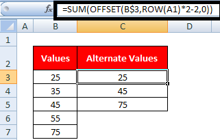
Suppose data starts from cell B3 (as shown in the image above). Type the following formula in cell C3.
ROW Function
It returns the row number of a reference.
Examples :
=SUM(OFFSET($A$1,0,0,COLUMN(B1)))
Evaluate Formula :
2. Rows - Number of rows you want Excel to move from the starting point.
3. Columns - Number of columns you want Excel to move from the starting point.
4. Height [Optional] - Size of range with number of rows tall you want to return.
5. Width [Optional] - Size of range with number of columns wide you want to return.
Examples :
1. OFFSET(A1,1,0)
It means move down 1 row i.e. A2. Since height and width components are optional in OFFSET formula, you can skip their references.
2. OFFSET(A1,0,2)
It means move right 2 columns i.e. C1.
3. OFFSET(A1,0,0,2)
From A1 returns 2 rows tall range. That means A1:A2
4. OFFSET(A1,0,0,1,2)
From A1 returns 2 columns wide range. That means A1:B1
5. OFFSET(A1,0,0,2,2)
From A1 returns 2 rows tall and 2 columns wide range. That means A1:B2
6. SUM(OFFSET(A1,1,2,2,1))
It means move down 1 row, 2 columns and then select 2 X 1 range. That means C2:C3
Real World Examples
Suppose you want to extract alternate values from a list.
Real World Examples
Suppose you want to extract alternate values from a list.
 |
| Excel OFFSET Function |
Suppose data starts from cell B3 (as shown in the image above). Type the following formula in cell C3.
=SUM(OFFSET(B$3,ROW(A1)*2-2,0))
ROW Function
It returns the row number of a reference.
Examples :
1. ROW(A1) returns 1.
2. ROW(A2) returns 2.
Scenario 2
Suppose you are asked to calculate cumulative sale. And the figure should be displayed in columns. Hence the formula should increment by row when you copy it horizontally.
Download the sample workbook
2. ROW(A2) returns 2.
Scenario 2
Suppose you are asked to calculate cumulative sale. And the figure should be displayed in columns. Hence the formula should increment by row when you copy it horizontally.
OFFSET - COLUMN
Evaluate Formula :
Let's translate the following formula into English :
=SUM(OFFSET($A$1,0,0,COLUMN(B1)))
Since COLUMN(B1) returns 2, the above formula means = SUM (A1 through 2 rows wide). That is equivalent to =SUM(A1:A3).
=SUM(OFFSET($A$1,0,0,COLUMN(B1)))
Since COLUMN(B1) returns 2, the above formula means = SUM (A1 through 2 rows wide). That is equivalent to =SUM(A1:A3).
When you copy the above formula across columns, the column formula increments by one.
=SUM(OFFSET($A$1,0,0,COLUMN(C1)))


Kindly notice the point you have mention:
ReplyDelete2. ROW(B1) returns 2.
--how can this is possible, as row return row number B1 is row 1, That means it will return 1 not 2.
--------------You Wrote--------------------------------------
ROW Function
It returns the row number of a reference.
Examples :
1. ROW(A1) returns 1.
2. ROW(B1) returns 2.
-------------------------------------------------
I think it's an error too Row(B1) Should return :1. Although i think he meant "A2" which should return 2.
ReplyDeleteTypo. Corrected!
ReplyDelete