Regression methods are widely used for predictive modeling. Most analytics professionals are familiar with only 2-3 common types such as linear and logistic regression. However, there are over 10 regression algorithms designed for different data and analyses. Understanding the right regression type based on data and distribution is important for effective analysis.

What is Regression Analysis?
In simple words, regression analysis is used to model the relationship between a dependent variable and one or more independent variables.
Lets take a simple example : Suppose your manager asked you to predict annual sales. There can be a hundred of factors (drivers) that affects sales. In this case, sales is your dependent variable. Factors affecting sales are independent variables. Regression analysis would help you to solve this problem.
It helps us to answer the following questions -
- Which of the drivers have a significant impact on sales
- Which is the most important driver of sales
- How do the drivers interact with each other
- What would be the annual sales next year.
Terminologies related to regression analysis
Suppose there is an observation in the dataset which is having a very high or very low value as compared to the other observations in the data, i.e. it does not belong to the population, such an observation is called an outlier. In simple words, it is extreme value. An outlier is a problem because many times it hampers the results we get.
When the independent variables are highly correlated to each other then the variables are said to be multicollinear. Many types of regression techniques assumes multicollinearity should not be present in the dataset. It is because it causes problems in ranking variables based on its importance. Or it makes job difficult in selecting the most important independent variable (factor).
When dependent variable's variability is not equal across values of an independent variable, it is called heteroscedasticity.
Example -As one's income increases, the variability of food consumption will increase. A poorer person will spend a rather constant amount by always eating inexpensive food; a wealthier person may occasionally buy inexpensive food and at other times eat expensive meals. Those with higher incomes display a greater variability of food consumption.
When we use unnecessary explanatory variables it might lead to overfitting. Overfitting means that our algorithm works well on the training set but is unable to perform better on the test sets. It is also known as problem of high variance.
When our algorithm works so poorly that it is unable to fit even training set well then it is said to underfit the data.It is also known as problem of high bias.
In the following diagram we can see that fitting a linear regression (straight line in fig 1) would underfit the data i.e. it will lead to large errors even in the training set. Using a polynomial fit in fig 2 is balanced i.e. such a fit can work on the training and test sets well, while in fig 3 the fit will lead to low errors in training set but it will not work well on the test set.
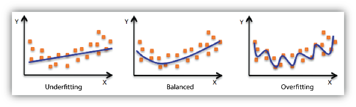 |
| Regression : Underfitting and Overfitting |
Types of Regression
Every regression technique has some assumptions attached to it which we need to meet before running analysis. These techniques differ in terms of type of dependent and independent variables and distribution.
1. Linear Regression
It is the simplest form of regression. It is a technique in which the dependent variable is continuous in nature. The relationship between the dependent variable and independent variables is assumed to be linear in nature.We can observe that the given plot represents a somehow linear relationship between the mileage and displacement of cars. The green points are the actual observations while the black line fitted is the line of regression.
 |
| Regression Analysis |
When you have only 1 independent variable and 1 dependent variable, it is called simple linear regression. When you have more than 1 independent variable and 1 dependent variable, it is called Multiple linear regression.
 |
Here 'y' is the dependent variable to be estimated, and X are the independent variables and ε is the error term. βi’s are the regression coefficients.
- There must be a linear relation between independent and dependent variables.
- There should not be any outliers present.
- No heteroscedasticity
- Sample observations should be independent.
- Error terms should be normally distributed with mean 0 and constant variance.
- Absence of multicollinearity and auto-correlation.
To estimate the regression coefficients βi’s we use principle of least squares which is to minimize the sum of squares due to the error terms i.e.
On solving the above equation mathematically we obtain the regression coefficients as:

Let us consider an example where the dependent variable is marks obtained by a student and explanatory variables are number of hours studied and no. of classes attended. Suppose on fitting linear regression we got the linear regression as:
Marks obtained = 5 + 2 (no. of hours studied) + 0.5(no. of classes attended)Thus we can have the regression coefficients 2 and 0.5 which can interpreted as:
- If no. of hours studied and no. of classes are 0 then the student will obtain 5 marks.
- Keeping no. of classes attended constant, if student studies for one hour more then he will score 2 more marks in the examination.
- Similarly keeping no. of hours studied constant, if student attends one more class then he will attain 0.5 marks more.
We consider the swiss data set for carrying out linear regression in R. We use lm() function in the base package. We try to estimate Fertility with the help of other variables.
library(datasets)
model = lm(Fertility ~ .,data = swiss)
lm_coeff = model$coefficients
lm_coeff
summary(model)
     (Intercept)      Agriculture      Examination        Education         Catholic
      66.9151817       -0.1721140       -0.2580082       -0.8709401        0.1041153
Infant.Mortality
       1.0770481


Call:
lm(formula = Fertility ~ ., data = swiss)
Residuals:
     Min       1Q   Median       3Q      Max
-15.2743  -5.2617   0.5032   4.1198  15.3213
Coefficients:
                 Estimate Std. Error t value Pr(>|t|)
(Intercept)      66.91518   10.70604   6.250 1.91e-07 ***
Agriculture      -0.17211    0.07030  -2.448  0.01873 *
Examination      -0.25801    0.25388  -1.016  0.31546
Education        -0.87094    0.18303  -4.758 2.43e-05 ***
Catholic          0.10412    0.03526   2.953  0.00519 **
Infant.Mortality  1.07705    0.38172   2.822  0.00734 **
---
Signif. codes:  0 ‘***’ 0.001 ‘**’ 0.01 ‘*’ 0.05 ‘.’ 0.1 ‘ ’ 1
Residual standard error: 7.165 on 41 degrees of freedom
Multiple R-squared:  0.7067, Adjusted R-squared:  0.671
F-statistic: 19.76 on 5 and 41 DF,  p-value: 5.594e-10
Hence we can see that 70% of the variation in Fertility rate can be explained via linear regression.
2. Polynomial Regression
It is a technique to fit a nonlinear equation by taking polynomial functions of independent variable.
In the figure given below, you can see the red curve fits the data better than the green curve. Hence in the situations where the relation between the dependent and independent variable seems to be non-linear we can deploy Polynomial Regression Models.

Thus a polynomial of degree k in one variable is written as:

Here we can create new features like
![]() and can fit linear regression in the similar manner.
and can fit linear regression in the similar manner.
In case of multiple variables say X1 and X2, we can create a third new feature (say X3) which is the product of X1 and X2 i.e.

Disclaimer: It is to be kept in mind that creating unnecessary extra features or fitting polynomials of higher degree may lead to overfitting.
We are using poly.csv data for fitting polynomial regression where we try to estimate the Prices of the house given their area.
Firstly we read the data using read.csv( )and divide it into the dependent and independent variable
data = read.csv("poly.csv")
x = data$Area
y = data$Price
In order to compare the results of linear and polynomial regression, firstly we fit linear regression:
model1 = lm(y ~x)
model1$fit
model1$coeffThe coefficients and predicted values obtained are:
       1        2        3        4        5        6        7        8        9       10
169.0995 178.9081 188.7167 218.1424 223.0467 266.6949 291.7068 296.6111 316.2282 335.8454

(Intercept)            x
120.05663769   0.09808581
We create a dataframe where the new variable are x and x square.
new_x = cbind(x,x^2) x
[1,] 500 250000
[2,] 600 360000
[3,] 700 490000
[4,] 1000 1000000
[5,] 1050 1102500
[6,] 1495 2235025
[7,] 1750 3062500
[8,] 1800 3240000
[9,] 2000 4000000
[10,] 2200 4840000model2 = lm(y~new_x)
model2$fit
model2$coeff
The fitted values and regression coefficients of polynomial regression are:
> model2$fit
       1        2        3        4        5        6        7        8        9       10
122.5388 153.9997 182.6550 251.7872 260.8543 310.6514 314.1467 312.6928 299.8631 275.8110
> model2$coeff
  (Intercept)        new_xx         new_x
-7.684980e+01  4.689175e-01 -1.402805e-04
Using ggplot2 package we try to create a plot to compare the curves by both linear and polynomial regression.
library(ggplot2)
ggplot(data = data) + geom_point(aes(x = Area,y = Price)) +
geom_line(aes(x = Area,y = model1$fit),color = "red") +
geom_line(aes(x = Area,y = model2$fit),color = "blue") +
theme(panel.background = element_blank())

3. Logistic Regression
In logistic regression, the dependent variable is binary in nature (having two categories). Independent variables can be continuous or binary. In multinomial logistic regression, you can have more than two categories in your dependent variable.
Here my model is:
 |
| logistic regression equation |
- Homoscedasticity assumption is violated.
- Errors are not normally distributed
- y follows binomial distribution and hence is not normal.
- HR Analytics : IT firms recruit large number of people, but one of the problems they encounter is after accepting the job offer many candidates do not join. So, this results in cost over-runs because they have to repeat the entire process again. Now when you get an application, can you actually predict whether that applicant is likely to join the organization (Binary Outcome - Join / Not Join).
- Elections : Suppose that we are interested in the factors that influence whether a political candidate wins an election. The outcome (response) variable is binary (0/1); win or lose. The predictor variables of interest are the amount of money spent on the campaign and the amount of time spent campaigning negatively.
Predicting the category of dependent variable for a given vector X of independent variables.Through logistic regression we have -
P(Y=1) = exp(a+ BₙX)/ (1+ exp(a+ BₙX))
Thus we choose a cut-off of probability say 'p' and if P(Yi = 1) > p then we can say that Yi belongs to class 1 otherwise 0.
If we take exponential of coefficients, then we’ll get odds ratio for ith explanatory variable. Suppose odds ratio is equal to two, then the odds of event is 2 times greater than the odds of non-event. Suppose dependent variable is customer attrition (whether customer will close relationship with the company) and independent variable is citizenship status (National / Expat). The odds of expat attrite is 3 times greater than the odds of a national attrite.
In this case, we are trying to estimate whether a person will have cancer depending whether he smokes or not.
We fit logistic regression with glm( )function and we setfamily = "binomial"
model <- glm(Lung.Cancer..Y.~Smoking..X.,data = data, family = "binomial")The predicted probabilities are given by:
#Predicted Probablities
model$fitted.values
        1         2         3         4         5         6         7         8         9
0.4545455 0.4545455 0.6428571 0.6428571 0.4545455 0.4545455 0.4545455 0.4545455 0.6428571
       10        11        12        13        14        15        16        17        18
0.6428571 0.4545455 0.4545455 0.6428571 0.6428571 0.6428571 0.4545455 0.6428571 0.6428571
       19        20        21        22        23        24        25
0.6428571 0.4545455 0.6428571 0.6428571 0.4545455 0.6428571 0.6428571
Predicting whether the person will have cancer or not when we choose the cut off probability to be 0.5.
data$prediction <- model$fitted.values>0.5> data$prediction
[1] FALSE FALSE TRUE TRUE FALSE FALSE FALSE FALSE TRUE TRUE FALSE FALSE TRUE TRUE TRUE
[16] FALSE TRUE TRUE TRUE FALSE TRUE TRUE FALSE TRUE TRUE
4. Quantile Regression
Quantile regression is the extension of linear regression and we generally use it when outliers, high skeweness and heteroscedasticity exist in the data.
In linear regression, we predict the mean of the dependent variable for given independent variables. Since mean does not describe the whole distribution, so modeling the mean is not a full description of a relationship between dependent and independent variables. So we can use quantile regression which predicts a quantile (or percentile) for given independent variables.
The term "quantile" is the same as "percentile"
In quantile regression we try to estimate the quantile of the dependent variable given the values of X's. Note : the dependent variable should be continuous.
Quantile regression model:
For qth quantile we have the following regression model:

This seems similar to linear regression model but here the objective function we consider to minimize is:
 where q is the qth quantile.
If q = 0.5 i.e. if we are interested in the median then it becomes median regression (or least absolute deviation regression) and substituting the value of q = 0.5 in above equation we get the objective function as:

Suppose the regression equation for 25th quantile of regression is:
y = 5.2333 + 700.823 x
It means that for one unit increase in x the estimated increase in 25th quantile of y by 700.823 units.
- Quite beneficial when heteroscedasticity is present in the data.
- Robust to outliers
- Distribution of dependent variable can be described via various quantiles.
- It is more useful than linear regression when the data is skewed.
It is to be kept in mind that the coefficients which we get in quantile regression for a particular quantile should differ significantly from those we obtain from linear regression. If it is not so then our usage of quantile regression isn't justifiable. This can be done by observing the confidence intervals of regression coefficients of the estimates obtained from both the regressions.
We need to install quantreg package in order to carry out quantile regression.
install.packages("quantreg")
library(quantreg)
Using rq function we try to predict the estimate the 25th quantile of Fertility Rate in Swiss data. For this we set tau = 0.25.
model1 = rq(Fertility~.,data = swiss,tau = 0.25)
summary(model1)
tau: [1] 0.25
Coefficients:
                 coefficients lower bd upper bd
(Intercept)      76.63132      2.12518 93.99111
Agriculture      -0.18242     -0.44407  0.10603
Examination      -0.53411     -0.91580  0.63449
Education        -0.82689     -1.25865 -0.50734
Catholic          0.06116      0.00420  0.22848
Infant.Mortality  0.69341     -0.10562  2.36095
Setting tau = 0.5 we run the median regression.
model2 = rq(Fertility~.,data = swiss,tau = 0.5)
summary(model2)
tau: [1] 0.5
Coefficients:
coefficients lower bd upper bd
(Intercept) 63.49087 38.04597 87.66320
Agriculture -0.20222 -0.32091 -0.05780
Examination -0.45678 -1.04305 0.34613
Education -0.79138 -1.25182 -0.06436
Catholic 0.10385 0.01947 0.15534
Infant.Mortality 1.45550 0.87146 2.21101We can run quantile regression for multiple quantiles in a single plot.
model3 = rq(Fertility~.,data = swiss, tau = seq(0.05,0.95,by = 0.05))
quantplot = summary(model3)
quantplot
We can check whether our quantile regression results differ from the OLS results using plots.
plot(quantplot)We get the following plot:

Various quantiles are depicted by X axis. The red central line denotes the estimates of OLS coefficients and the dotted red lines are the confidence intervals around those OLS coefficients for various quantiles. The black dotted line are the quantile regression estimates and the gray area is the confidence interval for themfor various quantiles. We can see that for all the variable both the regression estimated coincide for most of the quantiles. Hence our use of quantile regression is not justifiable for such quantiles. In other words we want that both the red and the gray lines should overlap as less as possible to justify our use of quantile regression.
5. Ridge Regression
It's important to understand the concept of regularization before jumping to ridge regression.
Regularization helps to solve over fitting problem which implies model performing well on training data but performing poorly on validation (test) data. Regularization solves this problem by adding a penalty term to the objective function and control the model complexity using that penalty term.
Regularization is generally useful in the following situations:
- Large number of variables
- Low ratio of number observations to number of variables
- High Multi-Collinearity
In L1 regularization we try to minimize the objective function by adding a penalty term to the sum of the absolute values of coefficients. This is also known as least absolute deviations method. Lasso Regression makes use of L1 regularization.
In L2 regularization we try to minimize the objective function by adding a penalty term to thesum of the squares of coefficients.RidgeRegression or shrinkage regression makes use of L2 regularization.
In general, L2 performs better than L1 regularization. L2 is efficient in terms of computation. There is one area where L1 is considered as a preferred option over L2. L1 has in-built feature selection for sparse feature spaces. For example, you are predicting whether a person is having a brain tumor using more than 20,000 genetic markers (features). It is known that the vast majority of genes have little or no effect on the presence or severity of most diseases.
In the linear regression objective function we try to minimize the sum of squares of errors. In ridge regression (also known as shrinkage regression) we add a constraint on the sum of squares of the regression coefficients. Thus in ridge regression our objective function is:

Here λ is the regularization parameter which is a non negative number. Here we do not assume normality in the error terms.
We do not regularize the intercept term. The constraint is just on the sum of squares of regression coefficients of X's.
We can see that ridge regression makes use of L2 regularization.
On solving the above objective function we can get the estimates of β as:
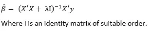
If we choose lambda = 0 then we get back to the usual OLS estimates. If lambda is chosen to be very large then it will lead to underfitting. Thus it is highly important to determine a desirable value of lambda.To tackle this issue, we plot the parameter estimates against different values of lambda and select the minimum value of λ after which the parameters tend to stabilize.
Considering the swiss data set, we create two different datasets, one containing dependent variable and other containing independent variables.
X = swiss[,-1]
y = swiss[,1]
We need to load glmnet library to carry out ridge regression.
library(glmnet)Using cv.glmnet( ) function we can do cross validation. By default alpha = 0 which means we are carrying out ridge regression. lambda is a sequence of various values of lambda which will be used for cross validation.
set.seed(123) #Setting the seed to get similar results.
model = cv.glmnet(as.matrix(X),y,alpha = 0,lambda = 10^seq(4,-1,-0.1))
best_lambda = model$lambda.min
ridge_coeff = predict(model,s = best_lambda,type = "coefficients")
ridge_coeff
The coefficients obtained using ridge regression are:
6 x 1 sparse Matrix of class "dgCMatrix"
                           1
(Intercept)      64.92994664
Agriculture      -0.13619967
Examination      -0.31024840
Education        -0.75679979
Catholic          0.08978917
Infant.Mortality  1.09527837
6. Lasso Regression
Lasso stands for Least Absolute Shrinkage and Selection Operator. It makes use of L1 regularization technique in the objective function. Thus the objective function in LASSO regression becomes:

λ is the regularization parameter and the intercept term is not regularized.
We do not assume that the error terms are normally distributed.
For the estimates we don't have any specific mathematical formula but we can obtain the estimates using some statistical software.
Note that lasso regression also needs standardization.
Lasso regression can perform in-built variable selection as well as parameter shrinkage. While using ridge regression one may end up getting all the variables but with Shrinked Paramaters.
Considering the swiss dataset from "datasets" package, we have:
#Creating dependent and independent variables.
X = swiss[,-1]
y = swiss[,1]
Using cv.glmnet in glmnet package we do cross validation. For lasso regression we set alpha = 1. By default standardize = TRUE hence we do not need to standardize the variables seperately.
#Setting the seed for reproducibility
set.seed(123)
model = cv.glmnet(as.matrix(X),y,alpha = 1,lambda = 10^seq(4,-1,-0.1))
#By default standardize = TRUE
We consider the best value of lambda by filtering out lamba.min from the model and hence get the coefficients using predict function.
#Taking the best lambda
best_lambda = model$lambda.min
lasso_coeff = predict(model,s = best_lambda,type = "coefficients")
lasso_coeff
The lasso coefficients we got are:
6 x 1 sparse Matrix of class "dgCMatrix"
1
(Intercept) 65.46374579
Agriculture -0.14994107
Examination -0.24310141
Education -0.83632674
Catholic 0.09913931
Infant.Mortality 1.07238898
Both ridge regression and lasso regression are addressed to deal with multicollinearity. Ridge regression is computationally more efficient over lasso regression.Any of them can perform better. So the best approach is to select that regression model which fits the test set data well.
7. Elastic Net Regression
Elastic Net regression is preferred over both ridge and lasso regression when one is dealing with highly correlated independent variables.
It is a combination of both L1 and L2 regularization.
The objective function in case of Elastic Net Regression is:

Like ridge and lasso regression, it does not assume normality.
Setting some different value of alpha between 0 and 1 we can carry out elastic net regression.
set.seed(123)
model = cv.glmnet(as.matrix(X),y,alpha = 0.5,lambda = 10^seq(4,-1,-0.1))
#Taking the best lambda
best_lambda = model$lambda.min
en_coeff = predict(model,s = best_lambda,type = "coefficients")
en_coeff
The coeffients we obtained are:
6 x 1 sparse Matrix of class "dgCMatrix"
                          1
(Intercept)      65.9826227
Agriculture      -0.1570948
Examination      -0.2581747
Education        -0.8400929
Catholic          0.0998702
Infant.Mortality  1.0775714
8. Principal Components Regression (PCR)
PCR is a regression technique which is widely used when you have many independent variables OR multicollinearity exist in your data. It is divided into 2 steps:
- Getting the Principal components
- Run regression analysis on principal components
The most common features of PCR are:
- Dimensionality Reduction
- Removal of multicollinearity
Principal components analysis is a statistical method to extract new features when the original features are highly correlated. We create new features with the help of original features such that the new features are uncorrelated.
Let us consider the first principal component:
The first PC is having the maximum variance. Similarly we can find the second PC U2 such that it is uncorrelated with U1 and has the second largest variance.
In a similar manner for 'p' features we can have a maximum of 'p' PCs such that all the PCs are uncorrelated with each other and the first PC has the maximum variance, then 2nd PC has the maximum variance and so on.
It is to be mentioned that PCR is not a feature selection technique instead it is a feature extraction technique. Each principle component we obtain is a function of all the features. Hence on using principal components one would be unable to explain which factor is affecting the dependent variable to what extent.
We use the longley data set available in R which is used for high multicollinearity. We excplude the Year column.
data1 = longley[,colnames(longley) != "Year"]This is how some of the observations in our dataset will look like:

We use pls packagein order to run PCR.
install.packages("pls")
library(pls)
pcr_model <- pcr(Employed~., data = data1, scale = TRUE, validation = "CV")
summary(pcr_model)
We get the summary as:
Data:  X dimension: 16 5
 Y dimension: 16 1
Fit method: svdpc
Number of components considered: 5
VALIDATION: RMSEP
Cross-validated using 10 random segments.
       (Intercept)  1 comps  2 comps  3 comps  4 comps  5 comps
CV           3.627    1.194    1.118   0.5555   0.6514   0.5954
adjCV        3.627    1.186    1.111   0.5489   0.6381   0.5819
TRAINING: % variance explained
          1 comps  2 comps  3 comps  4 comps  5 comps
X           72.19    95.70    99.68    99.98   100.00
Employed    90.42    91.89    98.32    98.33    98.74
Here in the RMSEP the root mean square errors are being denoted. While in 'Training: %variance explained' the cumulative % of variance explained by principle components is being depicted. We can see that with 3 PCs more than 99% of variation can be attributed.
We can also create a plot depicting the mean squares error for the number of various PCs.
validationplot(pcr_model,val.type = "MSEP")
By writing val.type = "R2" we can plot the R square for various no. of PCs.
validationplot(pcr_model,val.type = "R2")
If we want to fit pcr for 3 principal components and hence get the predicted values we can write:
pred = predict(pcr_model,data1,ncomp = 3)9. Partial Least Squares (PLS) Regression
It is an alternative technique of principal component regression when you have independent variables highly correlated. It is also useful when there are a large number of independent variables.
Both techniques create new independent variables called components which are linear combinations of the original predictor variables but PCR creates components to explain the observed variability in the predictor variables, without considering the response variable at all. While PLS takes the dependent variable into account, and therefore often leads to models that are able to fit the dependent variable with fewer components.
library(plsdepot)
data(vehicles)
pls.model = plsreg1(vehicles[, c(1:12,14:16)], vehicles[, 13], comps = 3)
# R-Square
pls.model$R2
10. Support Vector Regression
Support vector regression can solve both linear and non-linear models. SVM uses non-linear kernel functions (such as polynomial) to find the optimal solution for non-linear models.
The main idea of SVR is to minimize error, individualizing the hyperplane which maximizes the margin.
library(e1071)
svr.model <- svm(Y ~ X , data)
pred <- predict(svr.model, data)
points(data$X, pred, col = "red", pch=4)
11. Ordinal Regression
Ordinal Regression is used to predict ranked values. In simple words, this type of regression is suitable when dependent variable is ordinal in nature. Example of ordinal variables - Survey responses (1 to 6 scale), patient reaction to drug dose (none, mild, severe).
In linear regression, the dependent variable assumes that changes in the level of the dependent variable are equivalent throughout the range of the variable. For example, the difference in weight between a person who is 100 kg and a person who is 120 kg is 20kg, which has the same meaning as the difference in weight between a person who is 150 kg and a person who is 170 kg. These relationships do not necessarily hold for ordinal variables.
library(ordinal)
o.model <- clm(rating ~ ., data = wine)
summary(o.model)
12. Poisson Regression
Poisson regression is used when dependent variable has count data.
- Predicting the number of calls in customer care related to a particular product
- Estimating the number of emergency service calls during an event
- The dependent variable has a Poisson distribution.
- Counts cannot be negative.
- This method is not suitable on non-whole numbers
In the code below, we are using dataset named warpbreaks which shows the number of breaks in Yarn during weaving. In this case, the model includes terms for wool type, wool tension and the interaction between the two.
pos.model<-glm(breaks~wool*tension, data = warpbreaks, family=poisson)
summary(pos.model)
13. Negative Binomial Regression
Like Poisson Regression, it also deals with count data. The question arises "how it is different from poisson regression". The answer is negative binomial regression does not assume distribution of count having variance equal to its mean. While poisson regression assumes the variance equal to its mean.
When the variance of count data is greater than the mean count, it is a case of overdispersion. The opposite of the previous statement is a case of under-dispersion.
library(MASS)
nb.model <- glm.nb(Days ~ Sex/(Age + Eth*Lrn), data = quine)
summary(nb.model)
14. Quasi Poisson Regression
It is an alternative to negative binomial regression. It can also be used for overdispersed count data. Both the algorithms give similar results, there are differences in estimating the effects of covariates. The variance of a quasi-Poisson model is a linear function of the mean while the variance of a negative binomial model is a quadratic function of the mean.
qs.pos.model <- glm(Days ~ Sex/(Age + Eth*Lrn), data = quine, family = "quasipoisson")Quasi-Poisson regression can handle both over-dispersion and under-dispersion.
15. Cox Regression
Cox Regression is suitable for time-to-event data. See the examples below -
- Time from customer opened the account until attrition.
- Time after cancer treatment until death.
- Time from first heart attack to the second.
Logistic regression uses a binary dependent variable but ignores the timing of events.
As well as estimating the time it takes to reach a certain event, survival analysis can also be used to compare time-to-event for multiple groups.
Dual targets are set for the survival model
1. A continuous variable representing the time to event.
2. A binary variable representing the status whether event occurred or not.
library(survival)
# Lung Cancer Data
# status: 2=death
lung$SurvObj <- with(lung, Surv(time, status == 2))
cox.reg <- coxph(SurvObj ~ age + sex + ph.karno + wt.loss, data = lung)
cox.reg
16. Tobit Regression
It is used to estimate linear relationships between variables when censoring exists in the dependent variable.Censoring means when we observe independent variable for all observations, but we only know the true value of dependent variable for a restricted range of observations. Values of dependent in a certain range are reported as a single value. Detailed explanation of censoring is given below -
- Right censoring occurs when the event of interest does not occur before the end of study. The study can't wait for an event from a subject before the considered study period ends. Suppose you are building a customer attrition model in which dependent variable is binary (Attrited or still with the company).For those customers who are still with the company (not attrited) even when study ends (2 years) are right-censored.
- Left censoring is when the event of interest has already occurred before enrollment. This is very rarely encountered
- The Tobit model makes the same assumptions about error distributions as the OLS model, but it is much more vulnerable to violations of those assumptions.
- In an OLS model with heteroskedastic errors, the estimated standard errors can be too small
How to choose the correct regression model?
- If dependent variable is continuous and model is suffering from collinearity or there are a lot of independent variables, you can try PCR, PLS, ridge, lasso and elastic net regressions. You can select the final model based on Adjusted r-square, RMSE, AIC and BIC.
- If you are working on count data, you should try poisson, quasi-poisson and negative binomial regression.
- To avoid overfitting, we can use cross-validation method to evaluate models used for prediction. We can also use ridge, lasso and elastic net regressions techniques to correct overfitting issue.
- Try support vector regression when you have non-linear model.

Deepanshu founded ListenData with a simple objective - Make analytics easy to understand and follow. He has over 10 years of experience in data science. During his tenure, he worked with global clients in various domains like Banking, Insurance, Private Equity, Telecom and HR.
Should the part where you say "When you have more than 1 independent variable and 1 dependent variable, it is called simple linear regression" be multiple linear regression? It would be good to clarify because it comes right after "When you have only 1 independent variable and 1 dependent variable, it is called simple linear regression" and as a reader I would expect a contrast between the two blocks. Or if this is correct, a statement to validate that it is right after.
ReplyDeleteTypo. Corrected! Thanks for highlighting. Cheers!
DeleteThe piece is very good but some few regressions are left out. Beta regression, probit regression, tobit regression and probably a few others. For probit and tobit, it is just good to extend the treatise on logistic regression and try to explain their differences and when it might be preferable to use probit or tobit rather than logit. I have read a document where someone was trying to diffentiate between logistic regression and logit. I could not get the difference really, is there any at all? The comment by Vsoch is really important to correct.
ReplyDeleteWhat is the data set for Lung Cancer?
ReplyDeleteLoad survival package and then run command data(lung)
DeleteThis is great! I appreciate you explaining only what's necessary to inform a choice, but not defining all technical terms. I can look those up if I think a model's worth considering.
ReplyDeleteexcellent, very helpful, thank you.
ReplyDeleteWas there a reason that multinomial logistical regression was left out?
There is something a bit off with the definition here which you mentioned this and please correct me if I am wrong;
ReplyDeleteU said these
When we use unnecessary explanatory variables it might lead to overfitting. Overfitting means that our algorithm works well on the training set but is unable to perform better on the test sets. It is also known as problem of high variance.
When our algorithm works so poorly that it is unable to fit even training set well then it is said to underfit the data. It is also known as problem of high bias.
But I think when we overfit covariates into our models we would end up with a perfect model for the training data as you minimize the MSE which then also increases your bias towards the model which then increase the test MSE if you are able to test it using testing data
In my field of medical world I cannot do this training data usually cos it does not make sense
I am not sure if I understand right. For quantile regression the objective function is
ReplyDeleteq\sum | \eps_i | + (1-q) \sum | \eps_i | = \sum | \eps_i |.
Is this equation correct?
Hi, very good article yet there is a details you may correct if you want. The polynomial regression you are describing it is still a linear regression because the dependent variable, y, depend linearly on the regression coefficients. The fact the y is not linear versus x does not matter. From the practical point of view it means that with GNU R you can still use the "lm" function like in lm(y ~ x^2) and it will work as expected. The matrix computation of the linear regression and the matrix X is also still valid.
ReplyDeleteIn the elastic net regression I think there is a typo. There should be a + sign in between first and second terms of the equation on RHS
ReplyDeleteFor what type of dependent data, support vector regression is applicable? Is it applicable for the case when dependent variable is discrete and bounded?
ReplyDeleteDependent variable should be continuous in nature.
DeleteHello,
ReplyDeleteCan you please post some resources about how to deal with interactions in Regression using R? You have listed all kinds of regression models here. It would be great if you could cover Interactions and suggest how to interpret them. Maybe touching upon continuous, categorical, count and multilevel models. And giving some examples of real world data.
Is that possible?
Thanks,
Kunal
Hello, I used a Likert scale in a questionnaire and run a model where the dependent variable is the value of the answer. Using an ordinal regression model, 2 or 3 categories are "underranked". So my model results weak. Do you have any sugestion? Actually I could sum the value of the answers value for each interviewee obtaining a result from 3 to 15. What kind of model could I use in this case?
ReplyDeleteWhat is a Tobit regression model?
ReplyDeleteI have added it into this article. Thanks!
DeleteI was told we have more than fourth eight regression analysis. So my question goes to? can you help list and explain the rest of types
ReplyDeleteComprehensive article. One stop for regression models variance.
ReplyDeleteexcellent article
ReplyDeletegood information....is it possible to get the above information in pdf format. will highly appreciate
ReplyDeletehi Very good article. Do you have Python based examples. Please share if so
ReplyDeleteVery good article, you can also dd the multivariate regression model, extension of logistic regression. Otherwise it is a good piece of work.
ReplyDeleteThankyou as it's very consuming to give answers to these in the understanding
ReplyDeleteNice post
ReplyDeleteVery helpful article
ReplyDelete